Rendering of participating media is an important aspect of every modern renderer. When I say participating media, I am not just talking about fog, fire, and smoke. All matter is composed of atoms, which can be sparsely (e.g. in a gas) or densely (e.g. in a solid) distributed in space. Whether we consider the particle or the wave nature of light, it penetrates all matter (even metals) to a certain degree and interacts with its atoms along the way. The nature and the degree of “participation” depend on the material in question.
In the radiative transfer literature, light-material interaction is usually quantified in terms of absorption (conversion of electromagnetic energy of photons into kinetic energy of atoms, which manifests itself as reduction of light intensity) and scattering (absorption followed by emission of electromagnetic energy on collision). Therefore, it is common to describe participating media using the collision coefficients: the absorption coefficient \(\beta_a\) and the scattering coefficient \(\beta_s\). These coefficients give the probability density of the corresponding event per unit distance traveled by a photon, which implies the SI unit of measurement is \(m^{-1}\).
The extinction coefficient \(\beta_t\)
$$ \tag{1} \beta_t = \beta_a + \beta_s $$
gives the probability density of absorption or scattering (or, in other words, the collision rate) as a photon travels a unit distance through the medium1.
A more artist-friendly parametrization uses the single-scattering albedo \(\alpha_{ss}\)
$$ \tag{2} \alpha_{ss} = \frac{\beta_s}{\beta_t}, $$
which gives the deflection probability (or, in other words, the scattering rate), and the mean free path \(d\)
$$ \tag{3} d = \frac{1}{\beta_t}, $$
which corresponds to the average collision-free (or free-flight) distance.
It’s worth noting that the absorption coefficient is directly related to the attenuation index \(\kappa\), which is the imaginary part of the complex refractive index (IOR) \(\eta - i \kappa\):
$$ \tag{4} \kappa = \frac{\lambda}{4 \pi} \beta_a. $$
Note that, in this context, I am not talking about the IOR of an individual microscopic particle (which influences the microscopic scattering process), but rather about the properties of the macroscopic medium (composed of many microscopic particles).
The tuple \(\lbrace \eta, \kappa, \beta_s \rbrace\) \(\big(\)or, alternatively, \(\lbrace \eta, d, \alpha_{ss} \rbrace \big) \) contains sufficient information to describe both the behavior at the surface (boundary) and the (isotropic) multiple-scattering process (known as subsurface scattering) inside the volume that ultimately gives rise to what we perceive as the surface albedo \(\alpha_{ms}\). Note that certain materials (metals, in particular) require modeling of wave interference to obtain expected reflectance values.
A surface, then, is just an optical interface signified by a discontinuity of optical properties of the medium (in reality, the transition at the boundary is continuous, with a thickness of several atomic layers, but we can ignore this fact at scales relevant to computer graphics).
Sometimes, it is convenient to specify the concentration (density) of the medium, and not its effective optical properties. For example, the extinction coefficient can be computed using the following formula:
$$ \tag{5} \beta_t = \rho \sigma_t, $$
where \(\rho\) is the mass density (measured in units of \(kg/m^{3}\)) and \(\sigma_t\) is the mass extinction coefficient (in units of \(m^{2}/kg\)) - effective cross section per unit mass2. Other coefficients have the same linear relation with density.
But what about the IOR? Often, we assume that it is independent of density. But, if you consider water and steam (which has a lower concentration of water molecules), our experience tells us that their refractive properties are not the same.
There are several known relations between density and the IOR. One of them is given by the Lorentz–Lorenz equation:
$$ \tag{6} \frac{\eta^2 - 1}{\eta^2 + 2} = \frac{1}{3} \frac{\rho}{m} \frac{\alpha_m}{\varepsilon_0}, $$
where \(m\) is the molecular mass (in \(kg\)), \(\varepsilon_0\) is the vacuum permittivity, and \(\alpha_m\) is the mean molecular polarizability (SI units of \(C m^{2}/V\), watch out for different conventions). Since it is related to the complex IOR, polarizability is also complex. Incidentally, this equation presents a way to compute the IOR of a mixture of several substances. The corresponding Lorentz–Lorenz mixture rule is based on four principles of additivity (namely, of mole, mass, volume, and molecular polarizability, with the last two assumption being rather context-dependent).
For materials with small mass densities, the molecules are far apart, the molecular interactions are weak, and the IOR is close to 1. Therefore, for matter in the gas state, the following approximation can be made:
$$ \begin{aligned} \tag{7} \eta^2 & \approx 1 + \frac{\rho}{m} \frac{\alpha_m}{\varepsilon_0} = 1 + 2 \rho \delta_c, \cr \eta & \approx 1 + \frac{\rho}{2 m} \frac{\alpha_m}{\varepsilon_0} = 1 + \rho \delta_c, \end{aligned} $$
where \(\delta_c\) is the light dispersion coefficient. This equation implies that the relative brake power \((\eta - 1)\) has an approximately linear relation with density. Similar relations can be found for temperature and and pressure (in fact, all coefficients are highly temperature-dependent). Also, while the discussion above mostly concerns dielectrics, the formula for metals is very similar.
Continuous variation of the IOR poses many challenges for path tracing. In piecewise-uniform media, paths are composed of straight segments joined at scattering locations. Unfortunately, due to Fermat’s principle, continuously varying IOR forces photons to travel along paths of least time that bend towards regions of higher density according to Snell’s law. This fact alone makes basic actions like visibility testing quite complicated. And since the IOR may depend on the frequency, it can cause dispersion not only at the interfaces, but also continuously, along the entire path. Finally, one must model losses and gains due to continuous reflection/transmission, which is mathematically challenging. So it is not too surprising that most renderers ignore this behavior (even though, physically, that doesn’t make much sense). For small density gradients and small distances, it is a valid approximation that, on average, gives reasonably accurate results. On the other hand, for certain atmospheric effects, atmospheric refraction and reflection make a non-negligible contribution.
For practical reasons, further discussion will use a (typical) assumption that, within volume boundaries, the IOR is invariant with respect to position. If you are interested in continuous refraction, I encourage you to check out the Refractive Radiative Transfer Equation paper.
Radiative Transfer Equation
Intelligent sampling of a function requires understanding which parts make a large contribution. Therefore, we must briefly discuss the radiative transfer equation (or RTE) used to render scenes with participating media. While the full derivation is outside the scope of this article, we will try to touch the important aspects.
The integral form of the RTE is that of a recursive line integral. Intuitively, it models the process of photons traveling along the ray from sources towards the sensor, while at the same time accounting for energy losses.
These losses are primarily expressed by the opacity term \(O\), which is defined as the fraction of photons (quantified as radiance \(L\)) lost along the ray from \(\bm{x}\) to \(\bm{y}\) due to absorption and out-scattering:
$$ \tag{8} O(\bm{x}, \bm{y}) = \frac{L(\bm{y}, \bm{v}) - L(\bm{x}, \bm{v})}{L(\bm{y}, \bm{v})} = 1 - \frac{L(\bm{x}, \bm{v})}{L(\bm{y}, \bm{v})}, $$
where \(\bm{v} = (\bm{x} - \bm{y})/ \vert \bm{x} - \bm{y} \vert \) is the normalized view direction. Intuitively, \(O(\bm{x}, \bm{y}) = O(\bm{y}, \bm{x})\).
Its complement is transmittance \(T\):
$$ \tag{9} T(\bm{x}, \bm{y}) = 1 - O(\bm{x}, \bm{y}). $$
For a single photon, transmittance gives the probability of a free flight.
Volumetric transmittance is given by the Beer–Lambert–Bouguer law for uncorrelated media in terms of optical depth (or optical thickness) \(\tau\), which is a line integral from \(\bm{x}\) to \(\bm{y}\):
$$ \tag{10} \tau(\bm{x}, \bm{y}) = -\log{T(\bm{x}, \bm{y})} = \int_{\bm{x}}^{\bm{y}} \beta_t(\bm{u}) d\beta(\bm{u}) = \int_{\bm{x}}^{\bm{y}} \beta_t(\bm{u}) du, $$
where \(\bm{u} = \bm{x} - u \bm{v}\) is the point at the distance \(u\) along the ray, and \(du\) is the length measure associated with \(\bm{u}\). This formula implies that while transmittance is multiplicative, with values restricted to the unit interval, optical depth is additive and can take on any non-negative value. In other words, transmittance is a product integral:
$$ \tag{11} T(\bm{x}, \bm{y}) = e^{- \int_{\bm{x}}^{\bm{y}} \beta_t(\bm{u}) du} = \prod_{\bm{x}}^{\bm{y}} \Big( 1 - \beta_t(\bm{u}) du \Big). $$
Other integral formulations of volumetric transmittance exist.
The RTE models three types of energy sources: volumetric emission \(L_e\), volumetric in-scattering \(L_s\), and surface in-scattering \(L_g\) (which is itself an integral that features a surface geometry term with a BSDF). The volumetric in-scattering term \(L_s\) is an integral over \(4 \pi\) steradians:
$$ \tag{12} L_s(\bm{x}, \bm{v}) = \int_{4 \pi} \alpha_{ss}(\bm{x}) \frac{f_p(\bm{x}, \bm{v}, \bm{l})}{4 \pi} L(\bm{x}, \bm{l}) d\Omega_l, $$
where \(f_p\) denotes the phase function which models the angular distribution of scattered light3, and \(d\Omega_l\) is the solid angle measure associated with \(\bm{l}\).
Carefully putting it all together yields the volume rendering equation along the ray \(\bm{u} = \bm{x} - u \bm{v}\):
$$ \tag{13} L(\bm{x}, \bm{v}) = T(\bm{x}, \bm{y}) L_g(\bm{y}, \bm{v}) + \int_{\bm{x}}^{\bm{y}} T(\bm{x}, \bm{u}) \Big( \beta_a(\bm{u}) L_e(\bm{u}, \bm{v}) + \beta_t(\bm{u}) L_s(\bm{u}, \bm{v}) \Big) du $$
where \(\bm{y}\) denotes the position of the closest surface along the ray4.
We will leave volumetric emission out by setting \(L_e = 0\):
$$ \tag{14} L(\bm{x}, \bm{v}) = T(\bm{x}, \bm{y}) L_g(\bm{y}, \bm{v}) + \int_{\bm{x}}^{\bm{y}} T(\bm{x}, \bm{u}) \beta_t(\bm{u}) L_s(\bm{u}, \bm{v}) du. $$
This integral can be evaluated using one of the Monte Carlo methods. The Monte Carlo estimator has the following form:
$$ \tag{15} L(\bm{x}, \bm{v}) \approx T(\bm{x}, \bm{y}) L_g(\bm{y}, \bm{v}) + \frac{1}{N} \sum_{i=1}^{N} \frac{T(\bm{x}, \bm{u}_i) \beta_t(\bm{u}_i) L_s(\bm{u}_i, \bm{v})}{p( u_i | \lbrace \bm{x}, \bm{v} \rbrace)}, $$
where sample locations \(\bm{u}_i\) at the distance \(u_i\) along the ray are distributed according to the PDF \(p\).
We can importance sample the integrand (distribute samples according to the PDF) in several ways. Ideally, we would like to make the PDF proportional to the product of all terms of the integrand. However, unless we use path guiding, that is typically not possible. We will focus on the technique called free path sampling that makes the PDF proportional to the extinction-transmittance product \(T \beta_t\) (effectively, by assuming that the rest of the integrand varies slowly; in practice, this may or may not be the case - for example, for regions near light sources, equiangular sampling can give vastly superior results).
In order to turn the extinction-transmittance product into a PDF, it must be normalized over the domain of integration, \(\bm{x}\) to \(\bm{y}\). We must compute the normalization factor
$$ \tag{16} \int_{\bm{x}}^{\bm{y}} T(\bm{x}, \bm{u}) \beta_t(\bm{u}) du = \int_{\bm{x}}^{\bm{y}} e^{-\tau(\bm{x}, \bm{u})} \beta_t(\bm{u}) du. $$
If we use the fundamental theorem of calculus to interpret the extinction coefficient as a derivative
$$ \tag{17} \beta_t(\bm{u}) = \frac{\partial \tau}{\partial u}, $$
we can use the one of the exponential identities to simplify the extinction-transmittance integral:
$$ \tag{18} \int_{\bm{x}}^{\bm{y}} e^{-\tau(\bm{x}, \bm{u})} \frac{\partial \tau(\bm{x}, \bm{u})}{\partial u} du = -e^{-\tau(\bm{x}, \bm{u})} \Big\vert_{\bm{x}}^{\bm{y}} = 1 - T(\bm{x}, \bm{y}) = O(\bm{x}, \bm{y}). $$
Since it’s equal to opacity, the integral can be evaluated in a forward or backward fashion.
$$ \tag{19} \int_{\bm{x}}^{\bm{y}} e^{-\tau(\bm{x}, \bm{u})} \beta_t(\bm{u}) du = \int_{\bm{x}}^{\bm{y}} e^{-\tau(\bm{u}, \bm{y})} \beta_t(\bm{u}) du. $$
We can now define the normalized sampling PDF:
$$ \tag{20} p(u | \lbrace \bm{x}, \bm{v} \rbrace) = \frac{T(\bm{x}, \bm{u}) \beta_t(\bm{u})}{O(\bm{x}, \bm{y})}. $$
Substitution of the PDF into Equation 15 radically simplifies the estimator:
$$ \tag{21} L(\bm{x}, \bm{v}) \approx T(\bm{x}, \bm{y}) L_g(\bm{y}, \bm{v}) + O(\bm{x}, \bm{y}) \frac{1}{N} \sum_{i=1}^{N} L_s(\bm{u}_i, \bm{v}). $$
This equation can be seen as a form of premultiplied alpha blending (where alpha is opacity), which explains why particle cards can be so convincing. Additionally, it offers yet another way to parametrize the extinction coefficient - namely, by opacity at distance (which is similar to transmittance at distance used by Disney). It is the most RGB rendering friendly parametrization that I am aware of.
In this context, total opacity along the ray serves as the probability of a collision event within the medium, and can be used to make a random choice of the type of the sample (surface or volume):
$$ \tag{22} L(\bm{x}, \bm{v}) \approx \big(1 - O(\bm{x}, \bm{y}) \big) L_g(\bm{y}, \bm{v}) + O(\bm{x}, \bm{y}) \frac{1}{N} \sum_{i=1}^{N} L_s(\bm{u}_i, \bm{v}). $$
In order to sample the integrand of Equation 14, we must be also able to invert the CDF \(P\):
$$ \tag{23} P(u | \lbrace \bm{x}, \bm{v} \rbrace) = \int_{0}^{u} p(s | \lbrace \bm{x}, \bm{v} \rbrace) ds = \frac{O(\bm{x}, \bm{u})}{O(\bm{x}, \bm{y})}. $$
In practice, this means that we need to solve for the distance \(u\) given the value of optical depth \(\tau\):
$$ \tag{24} \tau(\bm{x}, \bm{u}) = -\mathrm{log} \big( O(\bm{x}, \bm{u}) \big) = -\mathrm{log} \Big( 1 - P\big(u | \lbrace \bm{x}, \bm{v} \rbrace \big) O \big( \bm{x}, \bm{y} \big) \Big). $$
Types of Analytic Participating Media
If your background is in real-time rendering, you may have heard of constant, linear, and exponential fog. These names refer to the way density varies in space (typically, with respect to the altitude), and can be used to model effects like height fog and atmospheric scattering.
Uniform Density
This type of medium has uniform5 density across the entire volume:
$$ \tag{25} \rho = b. $$
This formulation makes computing optical depth easy (recall Equations 5 and 10):
$$ \tag{26} \tau(\bm{x}, \bm{u}) = \sigma_t \int_{\bm{x}}^{\bm{u}} \rho{(\bm{s})} ds = \sigma_t \int_{\bm{x}}^{\bm{u}} b ds = \sigma_t b \vert \bm{u} - \bm{x} \vert = \sigma_t b u. $$
The sampling “recipe” for the distance \(u\) is thus simply
$$ \tag{27} u = \frac{\tau}{\sigma_t b}, $$
which is consistent with previous work.
The resulting sampling algorithm is very simple:
- compute total opacity \(O \big( \bm{x}, \bm{y} \big)\) along the ray;
- generate a random CDF value \(P \big(u | \lbrace \bm{x}, \bm{v} \rbrace \big)\);
- compute optical depth \(\tau(\bm{x}, \bm{u})\) using Equation 24;
- compute the distance \(u\) using Equation 27.
Linear Variation of Density with Altitude (Plane-Parallel Atmosphere)
Without loss of generality, let’s assume that density varies with the third coordinate of the position \(\bm{x}\), which we interpret as the altitude. This is your typical “linear height fog on flat Earth” case:
$$ \tag{28} \rho(\bm{x}) = a h(\bm{x}) + b = a x_3 + b. $$
One can obtain homogeneous media by setting \(a = 0\).
We would like to evaluate the optical depth integral:
$$ \tag{29} \tau(\bm{x}, \bm{u}) = \sigma_t \int_{\bm{x}}^{\bm{u}} \rho{(\bm{s})} ds = \sigma_t \int_{\bm{x}}^{\bm{u}} \Big( a h(\bm{s}) + b \Big) ds. $$
In practice, it’s actually simpler to integrate with respect to the parametric coordinates of the ray:
$$ \tag{30} \tau(\bm{x}, \bm{v}, u) = \sigma_t \int_{0}^{u} \Big( a \big(x_3 - s v_3) + b \Big) ds = \sigma_t \Big( (a x_3 + b) - \frac{a v_3}{2} u \Big) u, $$
which is the product of the average extinction coefficient and the length of the interval, as expected.
The inversion process involves solving the quadratic equation for the distance \(u\):
$$ \tag{31} u = \frac{(a x_3 + b) \pm \sqrt{ (a x_3 + b)^2 - 2 a v_3 (\tau / \sigma_t)}}{a v_3}. $$
Physically, we are only interested in the smaller root (with the negative sign), since it gives the solution for positive density values. Note that uniform media \( \big( a v_3 = 0 \big) \) require special care.
Exponential Variation of Density with Altitude (Plane-Parallel Atmosphere)
We can replace the linear density function with an exponential:
$$ \tag{32} \rho(\bm{x}) = b e^{-h(\bm{x}) / H} = b e^{-x_3 / H}, $$
where \(H\) is the scale height, measured in meters. Another way to think about it is as of the reciprocal of the falloff exponent \(n\):
$$ \tag{33} \rho(\bm{x}) = b e^{-n x_3}. $$
Setting \(n = 0\) results in a uniform medium.
The expression of optical depth remains simple:
$$ \tag{34} \tau(\bm{x}, \bm{v}, u) = \sigma_t \int_{0}^{u} b e^{-n (x_3 - s v_3)} ds = \sigma_t b e^{-n x_3} \int_{0}^{u} e^{s n v_3} ds = \frac{\sigma_t b}{n v_3} e^{-n x_3} \Big( e^{n v_3 u} - 1 \Big). $$
Solving for the distance \(u\) is straightforward:
$$ \tag{35} u = \frac{1}{n v_3} \log \left(1 + \frac{\tau}{\sigma_t b} n v_3 e^{n x_3} \right). $$
Note that uniform media \( \big( n v_3 = 0 \big) \) require special care.
Sample code is listed below.
// 'height' is the altitude.
// 'cosTheta' is the Z component of the ray direction.
// 'dist' is the distance.
// seaLvlExt = (sigma_t * b) is the sea-level (height = 0) extinction coefficient.
// n = (1 / H) is the falloff exponent, where 'H' is the scale height.
spectrum OptDepthRectExpMedium(float height, float cosTheta, float dist,
                               spectrum seaLvlExt, float n)
{
    float p = -cosTheta * n;

    // Equation 26.
    spectrum optDepth = seaLvlExt * dist;

    if (abs(p) > FLT_EPS) // Uniformity check
    {
        // Equation 34.
        optDepth = seaLvlExt * rcp(p) * exp(height * n) * (exp(p * dist) - 1);
    }

    return optDepth;
}

// 'optDepth' is the value of optical depth.
// 'height' is the altitude.
// 'cosTheta' is the Z component of the ray direction.
// seaLvlExtRcp = (1 / seaLvlExt).
// n = (1 / H) is the falloff exponent, where 'H' is the scale height.
float SampleRectExpMedium(float optDepth, float height, float cosTheta,
                          float seaLvlExtRcp, float n)
{
    float p = -cosTheta * n;

    // Equation 27.
    float dist = optDepth * seaLvlExtRcp;

    if (abs(p) > FLT_EPS) // Uniformity check
    {
        // Equation 35.
        dist = rcp(p) * log(1 + dist * p * exp(height * n));
    }

    return dist;
}
Exponential Variation of Density with Altitude (Spherical Atmosphere)
This is where things get interesting. We would like to model an exponential density distribution on a sphere:
$$ \tag{36} \rho(\bm{x}) = b e^{-h(\bm{x}) / H} = b e^{-(\vert \bm{x} - \bm{c} \vert - R) / H} = b e^{-n (\vert \bm{x} - \bm{c} \vert - R)}, $$
where \(\bm{c}\) is the center of the sphere, \(R\) is its radius, \(h\) is the altitude, and \(H\) is the scale height as before. In this context, \(b\) and \(\sigma_t b\) represent the density and the value of the extinction coefficient at the sea level, respectively. This formula gives the density of an isothermal atmosphere, which is not physically plausible.
Geometric Configuration of a Spherical Atmosphere
We can simplify the problem using its inherent spherical symmetry. Take a look at the diagram below.
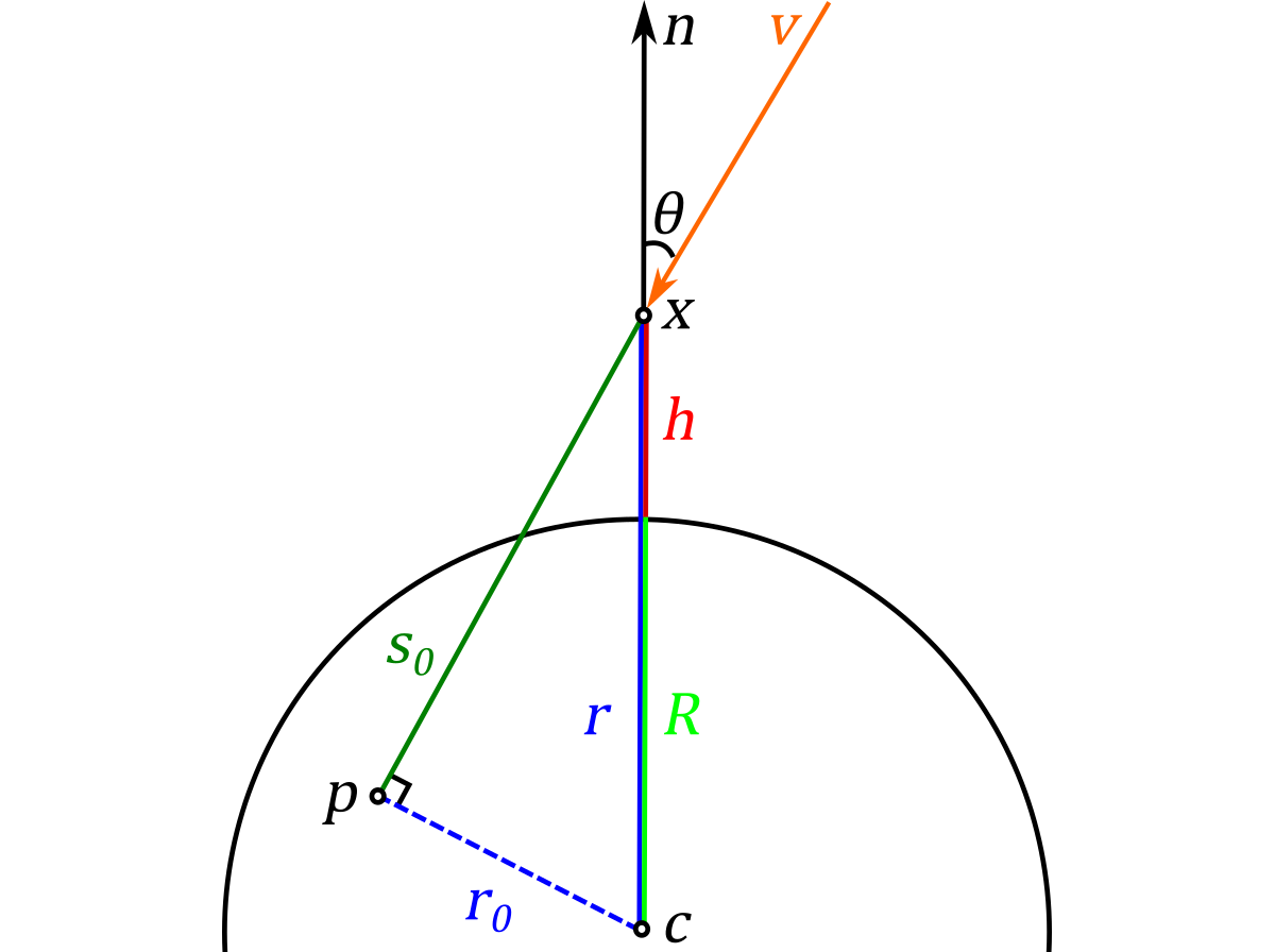
We start by recognizing the fact that every ordered pair of position and direction \(\lbrace \bm{x}, \bm{v} \rbrace\) can be reduced to a pair of radial distance and zenith angle \(\lbrace r, \theta \rbrace\), which means that our phase space is 2-dimensional.
In order to find the parametric equation of altitude \(h\) along the ray, we can use a right triangle with sides of length \(r_0\) and \(s_0\) corresponding to the initial position \(\bm{x}\):
$$ \tag{37} r_0 = r \sin{\theta}, \qquad s_0 = r \cos{\theta}. $$
This allows us to easily determine the radial distance and the zenith angle at any point along the ray.
$$ \tag{38} \mathcal{R}(r, \theta, s) = \sqrt{r_0^2 + (s_0 + s)^2} = \sqrt{(r \sin{\theta})^2 + (r \cos{\theta} + s)^2} = r \sqrt{1 + \frac{s}{r} \Big( 2 \cos{\theta + \frac{s}{r}} \Big)}. $$
$$ \tag{39} \mathcal{C}(r, \theta, s) = \frac{\mathrm{adjacent}}{\mathrm{hypotenuse}} = \frac{s_0 + s}{\mathcal{R}(r, \theta, s)} = \frac{\cos{\theta} + \frac{s}{r}}{\sqrt{1 + \frac{s}{r} \Big( 2 \cos{\theta + \frac{s}{r}} \Big)}}. $$
We can now compose the optical depth integral:
$$ \tag{40} \begin{aligned} \tau(r, \theta, u) &= \sigma_t b \int_{0}^{u} e^{-n h(s)} ds \cr &= \sigma_t b \int_{0}^{u} e^{-n \big( \mathcal{R}(r, \theta, s) - R \big)} ds \cr &= \sigma_t \frac{b}{n} e^{n (R - r)} \int_{0}^{u} e^{n \big( r - \mathcal{R}(r, \theta, s) \big)} n ds \cr &= \sigma_t \frac{b}{n} e^{n (R - r)} \int_{0}^{u} e^{n \big( r - \sqrt{r^2 + s (2 r \cos{\theta} + s)} \big)} n ds. \end{aligned} $$
The resulting integral is very complex. If we simplify using the following change of variables
$$ \tag{41} t = n s, \qquad z = n r, \qquad Z = n R $$
and change the upper limit of integration to infinity, we obtain what is known in the physics community as the Chapman’s grazing incidence integral (or the obliquity function, or the relative optical air mass) \(C\):
$$ \tag{42} C(z, \theta) = \int_{0}^{\infty} e^{z - \sqrt{z^2 + t (2 z \cos{\theta} + t)}} dt. $$
It is convenient to define the rescaled Chapman function \(C_r\)
$$ \tag{43} C_r(z, \theta) = e^{Z - z} C(z, \theta) = \int_{0}^{\infty} e^{Z - \sqrt{z^2 + t (2 z \cos{\theta} + t)}} dt, $$
which has a better numerical behavior, and further simplifies the expression of optical depth between \(\bm{x}\) and \(\bm{y}\):
$$ \tag{44} \tau(\bm{x}, \bm{y}) = \sigma_t \frac{b}{n} \Bigg( C_r \Big(z(\bm{x}), \cos{\theta(\bm{x})} \Big) - C_r \Big(z(\bm{y}), \cos{\theta(\bm{y})} \Big) \Bigg). $$
What Equation 44 tells us is that we should evaluate the optical depth integral twice (in the same direction, along the entire ray, from 0 to \(\infty\)), at the start and at the end of the interval, and subtract the results to “clip” the ray.
It is interesting to contemplate the physical meaning of optical depth and the Chapman function. Generally speaking, the value of a line integral of density (such as given by \(\tau / \sigma_t\)) corresponds to mass. Therefore, the integral
$$ \tag{45} \int_{h = (r - R)}^{\infty} b e^{-n s} ds = \frac{b}{n} e^{-n h} $$
gives the mass of an infinitely tall vertical column starting at the altitude \(h\). At the sea level, its mass is \(\frac{b}{n} = kH\).
Optical depth, then, is a product of the mass of the vertical column and the value of the obliquity function (which, intuitively, gives the absolute optical air mass along the oblique ray) times the mass extinction coefficient.
Examining the Chapman Function
It is always a good idea to examine a function visually, as a graph. Let’s do that.
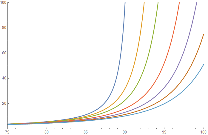
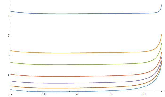
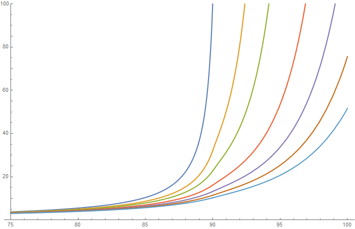
Plot of the Chapman function for r = 6600.
Above, I plotted values of the Chapman function (vertical axis) varying with the angle \(\theta\) (horizontal axis, in degrees) for different values of the scale height \(H\): \(1\) (blue), \(10\) (orange), \(20\) (green), \(40\) (red), \(60\) (purple), \(80\) (brown), \(100\) (light blue). Arguably, the first two are the most important, since they roughly correspond to scale heights of aerosols and air of Earth’s atmosphere. However, it is nice to be able to support larger values to model atmospheres of other planets.
Being an obliquity function, \(C(z, 0) = 1\). The function varies slowly, as long as the angle is far from being horizontal (which suggests an opportunity for a small angle approximation).
To my knowledge, the Chapman function does not have a closed-form expression. Many approximations exist. Unfortunately, most of them are specific to Earth’s atmosphere, and we are interested in a general solution. The most accurate approximation I have found was developed by David Huestis. He performs an asymptotic expansion in \(z\), which implies that his approximation becomes more accurate as the value of \(z\) increases (or, for fixed \(r\), as the value of \(H\) decreases). Using the first two terms results in the following formula for \(\theta \leq \pi/2\):
$$ \begin{aligned} \tag{46} C_u(z, \theta) &\approx \sqrt{\frac{1 - \sin{\theta}}{1 + \sin{\theta}}} \Bigg(1 - \frac{1}{2 (1 + \sin{\theta})} \Bigg) + \frac{\sqrt{\pi z}}{\sqrt{1 + \sin{\theta}}} \cr &\times \Bigg[ e^{z - z \sin{\theta}} \text{erfc}\left(\sqrt{z - z \sin{\theta}}\right) \Bigg] \Bigg( -\frac{1}{2} + \sin{\theta} + \frac{1}{1 + \sin{\theta}} + \frac{2 (1 + \sin{\theta}) - 1}{4 z (1 + \sin{\theta})} \Bigg). \end{aligned}$$
The approximation itself is also not closed-form, since it contains the complementary error function \(\mathrm{erfc}\). It’s also somewhat annoying that the result is given in terms of \(\sin{\theta}\) rather than \(\cos{\theta}\), but this reparametrization is actually necessarily to make the series converge quickly.
For the angle of 90 degrees, the integral is given using the modified Bessel function of the second kind \(K_1\):
$$ \tag{47} C_h(z) = C(z,\frac{\pi}{2}) = z e^z K_1(z) \approx \sqrt{\frac{\pi z}{2}} \left(1 + \frac{3}{8 z} -\frac{15}{128 z^2}\right). $$
We use a slightly more accurate approximation than \(C_u(z, \pi/2)\) to obtain some extra precision near 0 (we add the quadratic term).
Beyond the 90 degree angle, the following identity can be used:
$$ \tag{48} C_l(z, \theta) = 2 C_h(z \sin{\theta}) e^{z - z \sin{\theta}} - C_u(z, \pi - \theta), $$
which means that we must find a position \(\bm{p}\) (sometimes called the periapsis point, see the diagram in the previous section) along the ray where it is orthogonal to the surface normal, evaluate the horizontal Chapman function there (twice, forward and backward, to cover the entire real line), and subtract the value of the Chapman function at the original position with the reversed direction (towards the atmospheric boundary), which isolates the integral to the desired ray segment.
Sample implementation is listed below.
float ChapmanUpper(float z, float absCosTheta)
{
    float sinTheta = sqrt(saturate(1 - absCosTheta * absCosTheta));

    float zm12 = rsqrt(z);           // z^(-1/2)
    float zp12 = z * zm12;           // z^(+1/2)

    float tp   = 1 + sinTheta;       // 1 + Sin
    float rstp = rsqrt(tp);          // 1 / Sqrt[1 + Sin]
    float rtp  = rstp * rstp;        // 1 / (1 + Sin)
    float stm  = absCosTheta * rstp; // Sqrt[1 - Sin] = Abs[Cos] / Sqrt[1 + Sin]
    float arg  = zp12 * stm;         // Sqrt[z - z * Sin], argument of Erfc
    float e2ec = Exp2Erfc(arg);      // Exp[x^2] * Erfc[x]

    // Term 1 of Equation 46.
    float mul1 = absCosTheta * rtp;  // Sqrt[(1 - Sin) / (1 + Sin)] = Abs[Cos] / (1 + Sin)
    float trm1 = mul1 * (1 - 0.5 * rtp);

    // Term 2 of Equation 46.
    float mul2 = SQRT_PI * rstp * e2ec; // Sqrt[Pi / (1 + Sin)] * Exp[x^2] * Erfc[x]
    float trm2 = mul2 * (zp12 * (-1.5 + tp + rtp) +
                         zm12 * 0.25 * (2 * tp - 1) * rtp);
    return trm1 + trm2;
}

float ChapmanHorizontal(float z)
{
    float zm12 = rsqrt(z);           // z^(-1/2)
    float zm32 = zm12 * zm12 * zm12; // z^(-3/2)

    float p = -0.14687275046666018 + z * (0.4699928014933126 + z * 1.2533141373155001);

    // Equation 47.
    return p * zm32;
}

// z = (r / H), Z = (R / H).
float RescaledChapman(float z, float Z, float cosTheta)
{
    float sinTheta = sqrt(saturate(1 - cosTheta * cosTheta));

    // Cos[Pi - theta] = -Cos[theta],
    // Sin[Pi - theta] =  Sin[theta],
    // so we can just use Abs[Cos[theta]].
    float ch = ChapmanUpper(z, abs(cosTheta)) * exp(Z - z); // Rescaling adds 'exp'

    if (cosTheta < 0)
    {
        // Ch[z, theta] = 2 * Exp[z - z_0] * Ch[z_0, Pi/2] - Ch[z, Pi - theta].
        // z_0 = r_0 / H = (r / H) * Sin[theta] = z * Sin[theta].
        float z_0 = z * sinTheta;
        float chP = ChapmanHorizontal(z_0) * exp(Z - z_0); // Rescaling adds 'exp'

        // Equation 48.
        ch = 2 * chP - ch;
    }

    return ch;
}
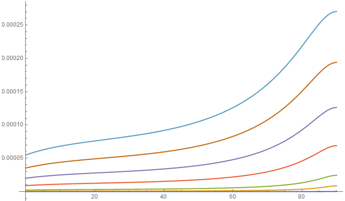
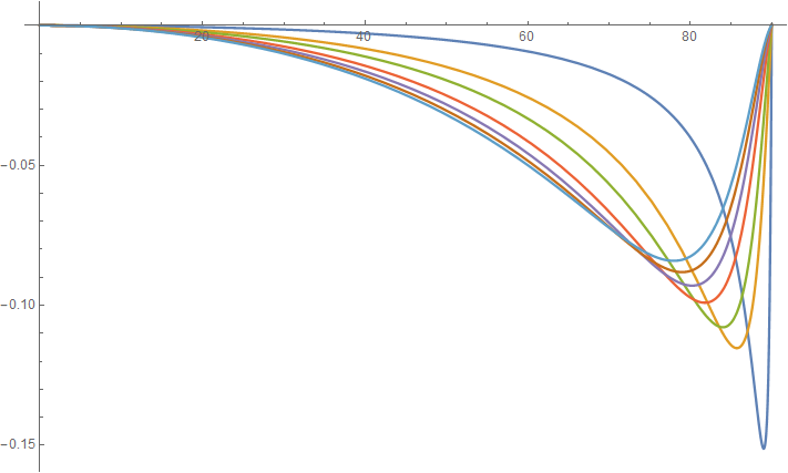
We can evaluate the quality of the approximation by computing the error with respect to the integral numerically evaluated in Mathematica.
Absolute error plot of the approximation of the Chapman function for r = 6600.
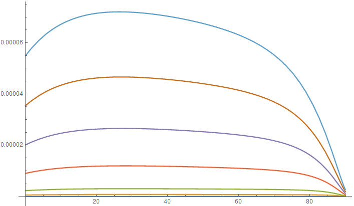
Relative error plot of the approximation of the Chapman function for r = 6600.
We can also represent the relative error as precision by plotting the number of digits after the decimal point. Since decimal precision of 32-bit floating numbers is between 6-8 digits, the approximation can be considered relatively accurate (particularly so for the range of typical values).
Precision plot of the approximation of the Chapman function for r = 6600.
Of course, we must address the elephant in the room, \(\mathrm{erfc}\). Since it is related to the normal distribution, it has numerous applications, and, as a result, dozens of existing approximations. Unfortunately, most of them are not particularly accurate, especially across a huge range of values (as in our case), and the accuracy of \(\mathrm{erfc}\) greatly affects the quality of our approximation.
After performing an extensive search, I stumbled upon the approximation developed by Takuya Ooura. He provides an impressive double-precision implementation accurate to 16 decimal digits. A great thing about his approximation is that it includes the \(\exp(x^2)\) factor, which means we can replace the entire term of Equation 46 inside the square brackets. In order to obtain a single-precision version of his approximation, I retain his range reduction technique and reduce the degree of the polynomial (which I fit using Sollya). In order to account for fused multiply-adds, I perform a greedy search for better coefficients (starting with single-precision coefficients found by Sollya) on the target hardware.
The implementation of Takuya Ooura (with my modifications) is reproduced below.
// Computes (Exp[x^2] * Erfc[x]) for (x >= 0).
// Range of inputs:  [0, Inf].
// Range of outputs: [0, 1].
// Max Abs Error: 0.000000969658452.
// Max Rel Error: 0.000001091639525.
float Exp2Erfc(float x)
{
    float t, u, y;

    t = 3.9788608f * rcp(x + 3.9788608f); // Reduce the range
    u = t - 0.5f;                         // Center around 0

    y =           -0.010297533124685f;
    y = fmaf(y, u, 0.288184314966202f);
    y = fmaf(y, u, 0.805188119411469f);
    y = fmaf(y, u, 1.203098773956299f);
    y = fmaf(y, u, 1.371236562728882f);
    y = fmaf(y, u, 1.312000870704651f);
    y = fmaf(y, u, 1.079175233840942f);
    y = fmaf(y, u, 0.774399876594543f);
    y = fmaf(y, u, 0.490166693925858f);
    y = fmaf(y, u, 0.275374621152878f);

    return y * t; // Expand the range
}
The approximation performs well, as you can see from the plots of the single-precision version shown below.
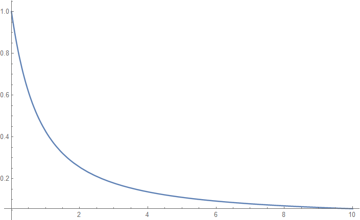
Plot of \(exp(x^2) erfc(x)\).
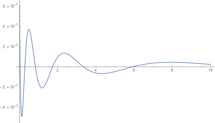
Absolute error plot of the approximation of \(exp(x^2) erfc(x)\).
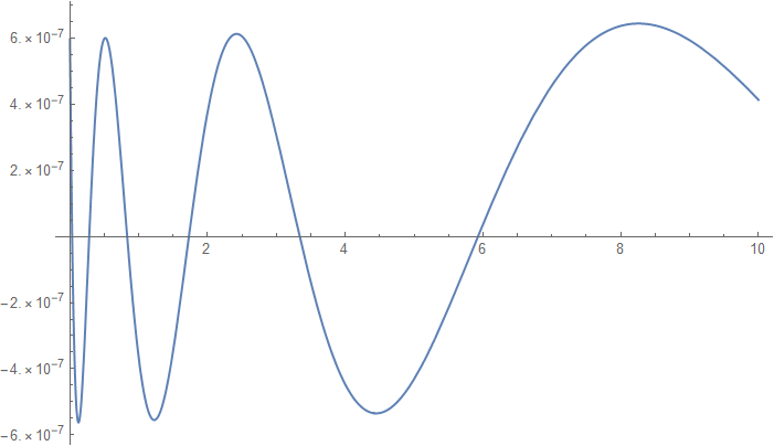
Relative error plot of the approximation of \(exp(x^2) erfc(x)\).
Since the error of this term is lower than the error of the approximation of the Chapman function, substituting the former does not visibly affect the error of the latter (and the error plots remain unchanged).
The proposed approximation is relatively expensive. It is particularly useful for path tracing, since the inversion process (described later) requires a certain degree of accuracy. If high accuracy is not required, you can (and probably should) use the approximation proposed by Christian Schüler in his GPU Gems 3 article:
$$ \tag{49} C_{cs}(z, \theta) \approx \frac{C_h(z)}{(C_h(z) - 1) \cos{\theta} + 1}. $$
It models the shape of the function pretty well, especially considering the cost.
Plot of the approximation of the Chapman function by Christian Schüler for r = 6600.
However, if you care about accuracy, and plot the relative error plot, it paints a slightly less attractive picture.
Relative error plot of the approximation of the Chapman function by Christian Schüler for r = 6600.
As always, there is a compromise. If you need accuracy (for a certain algorithm or technique), you must use a more accurate implementation. If every last cycle matters, it’s perfectly fine to “cheat” as long as the error is not very apparent.
I should also mention that Christian references another analytic expression of the Chapman function proposed by Miroslav Kocifaj. Miroslav’s paper has two equations of interest: one for arbitrary altitudes (11a), and one for small altitudes (11b), with the latter referenced in the GPU Pro article. Both look very similar to the power series expansion we are using, while at the same time featuring several orders of magnitude higher error (so both are clearly approximations, not exact solutions). Additionally, his formula for arbitrary altitudes depends on the planetary radius term (which can not be removed via simplification) which is not present in the integral formulation (Equation 42), which leads me to believe that the paper contains an error.
Evaluating Optical Depth Using the Chapman Function
A numerical approximation of the Chapman function, in conjunction with Equation 44, allows us to evaluate optical depth along an arbitrary ray segment.
However, the approximation of the Chapman function contains a branch (upper/lower hemisphere), and using the full formulation twice may be unnecessarily expensive for many use cases.
In order to evaluate optical depth between two arbitrary points \(\bm{x}\) and \(\bm{y}\), we have to consider three distinct possibilities:
1. \(\cos{\theta_x} \geq 0 \), which means that the ray points into the upper hemisphere with respect to the surface normal at the point \(\bm{x}\). This also means it points into the upper hemisphere at any point \(\bm{y}\) along the ray (that is fairly obvious if you sketch it). Optical depth is given by Equation 44, which we specialize by replacing \(C\) with \(C_u\), which is restricted to the upper hemisphere:
$$ \tag{50} \tau_{uu}(z_x, \theta_x, z_y, \theta_y) = \sigma_t \frac{b}{n} \Bigg( e^{Z - z_x} C_u(z_x, \theta_x) - e^{Z - z_y} C_u(z_y, \theta_y) \Bigg). $$
2. \(\cos{\theta_x} < 0 \) and \(\cos{\theta_y} < 0 \) occurs e.g. when looking straight down. It is also easy to handle, we just flip the direction of the ray (by taking the absolute value of the cosine), replace the segment \(\bm{xy}\) with the segment \(\bm{yx}\) and fall back to case 1.
3. \(\cos{\theta_x} < 0 \) and \(\cos{\theta_y} \geq 0 \). This is the most complicated case, since we have to evaluate the Chapman function three times, twice at \(\bm{x}\) and once at \(\bm{y}\):
$$ \tag{51} \begin{aligned} \tau_{lu}(z_x, \theta_x, z_y, \theta_y) &= \sigma_t \frac{b}{n} \Bigg( e^{Z - z_x} C_l(z_x, \theta_x) - e^{Z - z_y} C_u(z_y, \theta_y) \Bigg). \end{aligned} $$
Sample code is listed below.
float RadAtDist(float r, float rRcp, float cosTheta, float s)
{
    float x2 = 1 + (s * rRcp) * ((s * rRcp) + 2 * cosTheta);

    // Equation 38.
    return r * sqrt(x2);
}

float CosAtDist(float r, float rRcp, float cosTheta, float s)
{
    float x2 = 1 + (s * rRcp) * ((s * rRcp) + 2 * cosTheta);

    // Equation 39.
    return ((s * rRcp) + cosTheta) * rsqrt(x2);
}

// This variant of the function evaluates optical depth along an infinite path.
// 'r' is the radial distance from the center of the planet.
// 'cosTheta' is the value of the dot product of the ray direction and the surface normal.
// seaLvlExt = (sigma_t * b) is the sea-level (height = 0) extinction coefficient.
// 'R' is the radius of the planet.
// n = (1 / H) is the falloff exponent, where 'H' is the scale height.
spectrum OptDepthSpherExpMedium(float r, float cosTheta, float R,
                                spectrum seaLvlExt, float H, float n)
{
    float z = r * n;
    float Z = R * n;

    float ch = RescaledChapman(z, Z, cosTheta);

    return ch * H * seaLvlExt;
}

// This variant of the function evaluates optical depth along a bounded path.
// 'r' is the radial distance from the center of the planet.
// rRcp = (1 / r).
// 'cosTheta' is the value of the dot product of the ray direction and the surface normal.
// 'dist' is the distance.
// seaLvlExt = (sigma_t * b) is the sea-level (height = 0) extinction coefficient.
// 'R' is the radius of the planet.
// n = (1 / H) is the falloff exponent, where 'H' is the scale height.
spectrum OptDepthSpherExpMedium(float r, float rRcp, float cosTheta, float dist, float R,
                                spectrum seaLvlExt, float H, float n)
{
    float rX        = r;
    float rRcpX     = rRcp;
    float cosThetaX = cosTheta;
    float rY        = RadAtDist(rX, rRcpX, cosThetaX, dist);
    float cosThetaY = CosAtDist(rX, rRcpX, cosThetaX, dist);

    // Potentially swap X and Y.
    // Convention: at point Y, the ray points up.
    cosThetaX = (cosThetaY >= 0) ? cosThetaX : -cosThetaX;

    float zX  = rX * n;
    float zY  = rY * n;
    float Z   = R  * n;

    float chX = RescaledChapman(zX, Z, cosThetaX);
    float chY = ChapmanUpper(zY, abs(cosThetaY)) * exp(Z - zY); // Rescaling adds 'exp'

    // We may have swapped X and Y.
    float ch = abs(chX - chY);

    return ch * H * seaLvlExt;
}
Note that using this function (rather than calling OptDepthSpherExpMedium twice and subtracting the results) is beneficial not only for performance but also for correctness: it avoids numerical instability near the horizon where ray directions are prone to alternate between the two hemispheres, which could cause subtraction to result in negative optical depth values. For performance (and numerical stability) reasons, it may be also worth making a special case for when the point \(\bm{y}\) is far enough to be considered outside the atmosphere (if exp(Z - zY) < EPS, for instance). In that case, chY = 0 is an adequate approximation.
Sampling Exponential Media of a Spherical Atmosphere
One does not simply sample the Chapman function. There doesn’t appear to be a way to invert the integral formulation (Equation 40), and attempts at solving numerical approximations for distance seem futile. Of course, we still have the option to look for a numerical fit for the tabulated inverse, or to use a look-up table directly… But we are not going to do that. And here’s why.
In order to sample participating media, we must be able to solve the optical depth equation for distance. If you only have a single analytically-defined volume, sampling it is (usually) trivial. However, once you have several heterogeneous overlapping volumes, you start running into issues. While optical depth is additive, the sampled distance is not. So, what do we do?
If we can’t solve the equation analytically, we can solve it numerically, using the Newton–Raphson method. Recall that this method requires being able to make an initial guess, evaluate the function, and take its derivative. Our function is the total optical depth. We can make an initial guess by assuming that the combined medium is uniform (or, under certain assumptions, plane-parallel-exponential). And since we know that the derivative of optical depth is just the extinction coefficient \(\beta_t\) (see Equation 17), so we have all the pieces we need.
This method is very general and works for arbitrary continuous density distributions.
Sample code for a dual-component spherical atmosphere is listed below.
#define EPS_ABS  0.0001
#define EPS_REL  0.0001
#define MAX_ITER 4

// 'optDepth' is the value to solve for.
// 'maxOptDepth' is the maximum value along the ray, s.t. (maxOptDepth >= optDepth).
// 'maxDist' is the maximum distance along the ray.
float SampleSpherExpMedium(float optDepth, float r, float rRcp, float cosTheta, float R,
                           float2 seaLvlExt, float2 H, float2 n, // Air & aerosols
                           float maxOptDepth, float maxDist)
{
    const float  optDepthRcp = rcp(optDepth);
    const float2 Z           = R * n;

    // Make an initial guess (assume the medium is uniform).
    float t = maxDist * (optDepth * rcp(maxOptDepth));

    // Establish the ranges of valid distances ('tRange') and function values ('fRange').
    float tRange[2], fRange[2];
    tRange[0] = 0;        /* -> */  fRange[0] = 0           - optDepth;
    tRange[1] = maxDist;  /* -> */  fRange[1] = maxOptDepth - optDepth;

    uint  iter = 0;
    float absDiff = optDepth, relDiff = 1;

    do // Perform a Newton–Raphson iteration.
    {
        float radAtDist = RadAtDist(r, rRcp, cosTheta, t);
        float cosAtDist = CosAtDist(r, rRcp, cosTheta, t);
        // Evaluate the function and its derivatives:
        // f  [t] = OptDepthAtDist[t] - GivenOptDepth = 0,
        // f' [t] = ExtCoefAtDist[t],
        // f''[t] = ExtCoefAtDist'[t] = -ExtCoefAtDist[t] * CosAtDist[t] / H.
        float optDepthAtDist = 0, extAtDist = 0, extAtDistDeriv = 0;
        optDepthAtDist += OptDepthSpherExpMedium(r, rRcp, cosTheta, t, R,
                                                 seaLvlExt.x, H.x, n.x);
        optDepthAtDist += OptDepthSpherExpMedium(r, rRcp, cosTheta, t, R,
                                                 seaLvlExt.y, H.y, n.y);
        extAtDist      += seaLvlExt.x * exp(Z.x - radAtDist * n.x);
        extAtDist      += seaLvlExt.y * exp(Z.y - radAtDist * n.y);
        extAtDistDeriv -= seaLvlExt.x * exp(Z.x - radAtDist * n.x) * n.x;
        extAtDistDeriv -= seaLvlExt.y * exp(Z.y - radAtDist * n.y) * n.y;
        extAtDistDeriv *= cosAtDist;

        float   f = optDepthAtDist - optDepth;
        float  df = extAtDist;
        float ddf = extAtDistDeriv;
        float  dg = df - 0.5 * f * (ddf * rcp(df));

        assert(df > 0 && dg > 0);

    #if 0
        // https://en.wikipedia.org/wiki/Newton%27s_method
        float slope = rcp(df);
    #else
        // https://en.wikipedia.org/wiki/Halley%27s_method
        float slope = rcp(dg);
    #endif

        float dt = -f * slope;

        // Find the boundary value we are stepping towards:
        // supremum for (f < 0) and infimum for (f > 0).
        uint  sgn     = asuint(f) >> 31;
        float tBound  = tRange[sgn];
        float fBound  = fRange[sgn];
        float tNewton = t + dt;

        bool isInRange = tRange[0] < tNewton && tNewton < tRange[1];

        if (!isInRange)
        {
            // Newton's algorithm has effectively run out of digits of precision.
            // While it's possible to continue improving precision (to a certain degree)
            // via bisection, it is costly, and the convergence rate is low.
            // It's better to recall that, for short distances, optical depth is a
            // linear function of distance to an excellent degree of approximation.
            slope = (tBound - t) * rcp(fBound - f);
            dt    = -f * slope;
            iter  = MAX_ITER;
        }

        tRange[1 - sgn] = t; // Adjust the range using the
        fRange[1 - sgn] = f; // previous values of 't' and 'f'

        t = t + dt;

        absDiff = abs(optDepthAtDist - optDepth);
        relDiff = abs(optDepthAtDist * optDepthRcp - 1);

        iter++;

        // Stop when the accuracy goal has been reached.
        // Note that this uses the accuracy corresponding to the old value of 't'.
        // The new value of 't' we just computed should result in higher accuracy.
    } while ((absDiff > EPS_ABS) && (relDiff > EPS_REL) && (iter < MAX_ITER));

    return t;
}
Since optical depth is a smooth monotonically increasing function of distance, this numerical procedure will converge very quickly (typically, after a couple of iterations). If desired, the cost can be fixed by using an iteration counter to terminate the loop, potentially trading accuracy for consistent performance.
It is worth noting that since the code internally uses a numerical approximation of the Chapman function, it may not always be possible to reach an arbitrary accuracy goal. Once the algorithm becomes numerically unstable, we refine the result by assuming that the medium is approximately uniform along short intervals.
In fact, the curvature of the planet can be ignored for moderate distances, making the rectangular inverse a relatively efficient and accurate approximation.
Conclusion
This article has presented several methods for sampling common types of analytic participating media. They are particularly useful for modeling low-frequency variations of density. While planetary atmospheres cannot be sampled analytically, the proposed numerical approach works well in practice. None of these techniques require voxelization, which allows simulation of various volumetric effects at real-time frame rates.
Acknowledgments
I would like to thank Julian Fong and Sébastien Hillaire for their thoughtful comments and feedback.
-
According to Wikipedia, this is an old term, and we should refer to it as the attenuation coefficient instead. While it’s certainly a better name, in practice, all classical publications call it extinction (this also includes related terms). We use the classical naming convention to avoid confusion. ↩︎
-
Alternatively, one can use number density instead of mass density. ↩︎
-
Certain authors use the definition of the phase function that includes the albedo. ↩︎
-
The absorption coefficient in front of the emission term is due to the Kirchhoff’s law which states that, for an arbitrary body emitting and absorbing thermal radiation in thermodynamic equilibrium, the emissivity is equal to the absorptivity. ↩︎
-
A homogeneous medium, by definition, contains no inhomogeneities (which cause scattering), while a medium with a uniform density is composed of scattering particles. ↩︎