Deep Compositing and Reprojection

Most graphics programmers are familiar with the concept of alpha. It has two interpretations - geometrical and optical. The former corresponds to coverage, while the latter refers to opacity.

Regular compositing assumes non-overlapping objects. Typically, the over operator is used. It implies that one of the objects is in front of the other, and thereby attenuates its contribution to the image.

This blog post will cover deep compositing.

It assumes the optical interpretation of alpha, and implies that objects overlap within a certain depth interval (e.g. along the ray).

As the name implies, the technique can be used to composite volumetric effects stored in 3D texture AOVs, such as renders of clouds or smoke.

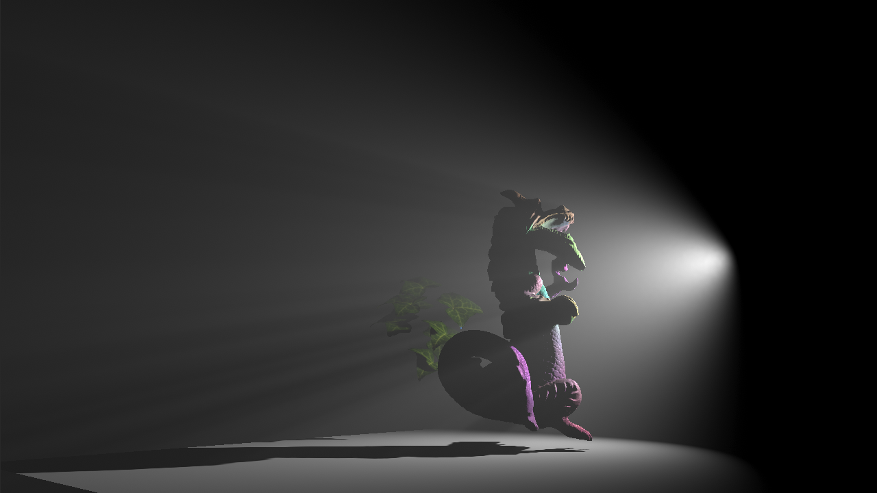
Another notable application is temporal reprojection for voxel-based volumetric lighting. As detailed in my Siggraph 2018 presentation, one way of performing temporal integration of volumetrics is to compute ray sub-integrals (along with associated opacity), store them in a 3D texture, and then look them up during the next frame. This involves both resampling (filtering) and rescaling, and both of these operations must be linear in order to not cause artifacts such as unexpected changes in brightness during camera motion.

Deep compositing is a solved problem. The paper by Tom Duff gives a detailed description of the algorithm, the mathematics involved, as well as several applications.

To sum it up, a deep pixel or voxel (represented as a pair of color and opacity) is assumed to be in the exp space. To ensure that filtering and compositing operations are linear, they should operate on log-transformed values.

The transformations are given as follows:

OpticalDepthFromOpacity(a) = -log(1 - a)
OpacityFromOpticalDepth(d) = 1 - exp(-d)

log(X) = {OpticalDepthFromOpacity( X.a) /  X.a * X.rgb, -OpticalDepthFromOpacity( X.a)}
exp(Y) = {OpacityFromOpticalDepth(-Y.a) / -Y.a * Y.rgb,  OpacityFromOpticalDepth(-Y.a)}

blend(A, B, t) = exp(lerp(log(A), log(B), t))

Note that you can drop negations from the definitions of log(X) and exp(Y) for convenience.

If you take a look at the derivation in Tom’s paper, it assumes that both pixels taking part in the blend operation correspond to objects overlapping the same depth interval. This presents a problem in the context of voxel-based volumetrics, since voxels sizes can vary dramatically, making blending of voxels corresponding to different depth intervals (of different sizes) a requirement to support reprojection during camera motion.

In my Siggraph talk, I proposed a solution, which is to linearize pixels with respect to the size of the interval, normalize them (divide by the size), and then use Tom’s blending algorithm. While the idea was conceptually sound, I wasn’t able to find the correct solution for linearization and normalization before the conference deadline, and ended up presenting an ad-hoc method instead.

Turns out, the correct solution is very simple, and requires no additional transformations. Tom’s log transform actually performs linearization - this is why he is able to use the linear interpolation formula. It’s possible to reason about this mathematically, but I found thinking about the physical interpretation of the transformation more intuitive.

Given a homogeneous participating medium under constant illumination, the value of the in-scattered radiance integral along the ray segment (which is identical to the weight given by free-path sampling in the Monte Carlo context) is proportional to:

L_o = c * L_i * OpacityFromOpticalDepth(k * x) / k

where k is the extinction coefficient and x is the length of the interval. Their product is the optical depth d.

The full value of the pixel P (including its opacity) is thus:

P = {c * L_i * OpacityFromOpticalDepth(k * x) / k, OpacityFromOpticalDepth(k * x)}

Let’s apply the log transform to P and simplify:

log(P) = {(k * x) / P.a * c * L_i * OpacityFromOpticalDepth(k * x) / k, -(k * x)}
log(P) = {c * L_i * x, -k * x}

As we can see, log(P) is a linear function of x, as well as of the incoming radiance L_i.

This makes the normalization operation trivial:

N = log(P) / x = {c * L_i, -k}

This quantity can be interpreted as density along (the unit interval of) the ray, represented as a pair of (rescaled) incoming radiance and extinction.

To sum up, linear blending of two pixels P_1 and P_2 of two different sizes x_1 and x_2 should be performed as follows:

1. Linearize: compute log(P_1) and log(P_2).
2. Normalize: compute N_1 = log(P_1) / x_1 and N_2 = log(P_2) / x_2.
3. Blend: compute B = lerp(N_1, N_2, t).
4. Denormalize: let’s say that (x_1 <= x_2) and we want to blend all of P_1 with a fraction of P_2 of size x_1. In that case, we compute B_1 = B * x_1.
5. Delinearize: convert back to color and opacity by computing E_1 = exp(B_1).

Despite the derivation assuming constant illumination, we apply the same technique to all light types (once per voxel, not once per light) with good results.

Acknowledgments

I would like to thank Sebastien Lagarde for reviewing this blog post and offering thoughtful comments.