Pre-filtered cubemaps remain an important source of indirect illumination for those of us who still haven’t purchased a Turing graphics card.
To my knowledge, most implementations use the split sum approximation originally introduced by Brian Karis. It is a simple technique, and generally works well given the inherent view independence limitation.
But why does it work so well, and is there a better way to pre-filter? Let’s find out.
To compute the outgoing radiance in the view direction, we need to evaluate the integral of the incoming radiance weighted by the BRDF over the projected hemisphere.
$$ L_o = \int_{\Omega} L_i(l) f(\alpha,v,n,l) \langle n,l \rangle dl $$
Brian’s solution is to split the integral in two:
$$ L_o \approx \int_{\Omega} L_i(l) \langle n,l \rangle dl \int_{\Omega} f(\alpha,v,n,l) \langle n,l \rangle dl $$
The first integral is stored in the pre-filtered cubemap, and is the biggest source of error, since it does not account for the view direction. The second integral can be precomputed and reconstructed exactly at runtime. In practice, during the cubemap pre-filtering step, Brian suggests to place samples according to the GGX distribution, which may be surprising given the absence of the BRDF within the integral.
We can do things slightly differently. Here is the way pre-filtering works in Unity’s HD Render Pipeline.
First, we note that we can compute the exact value of the second integral, so it makes perfect sense to keep it. Therefore, we can start with the following expression:
$$ L_o = L_p(\alpha,v,n) \int_{\Omega} f(\alpha,v,n,l) \langle n,l \rangle dl $$
After substituting into the first equation and solving for Lp, we arrive at the following expression:
$$ L_o = \frac{ \int_{\Omega} L_i(l) f(\alpha,v,n,l) \langle n,l \rangle dl }{ \int_{\Omega} f(\alpha,v,n,l) \langle n,l \rangle dl} \int_{\Omega} f(\alpha,v,n,l) \langle n,l \rangle dl $$
In this form, the IBL solution is exact. In practice, since we are memory-limited, we retain Brian’s approximation by assuming that the normal and the view vectors are aligned. This results in a normalized radially symmetric filter around the normal.
$$ L_p(\alpha,v,n) \approx \frac{ \int_{\Omega} L_i(l) f(\alpha,n,n,l) \langle n,l \rangle dl }{ \int_{\Omega} f(\alpha,n,n,l) \langle n,l \rangle dl} $$
It is now more clear why the pre-filtering step requires sampling according to the BRDF.
We can still evaluate both integrals (in the numerator and the denominator) using Monte-Carlo. After importance sampling (according to the NDF) and simplification, we arrive at the following expression:
$$ L_p(\alpha,v,n) \approx \frac{ \sum L_i(l) F(\langle h,l \rangle) G(\alpha,n,l) }{ \sum F(\langle h,l \rangle) G(\alpha,n,l) } = \frac{ \sum L_i(l) W }{ \sum W } $$
The only remaining snag is the Fresnel term, which depends both on the reflectance and the half-angle. Using
$$ F \approx const $$
will cause it to cancel out. I tried using the full Fresnel-Schlick expression with different reflectance values, and observed no visible difference in practice. At first, I was really puzzled as to why. Turns out, Fresnel-Schlick is nearly constant for angles up to 45 degrees, so this is indeed a reasonable approximation for most roughness values. My thanks to Brian for the explanation and the graph.
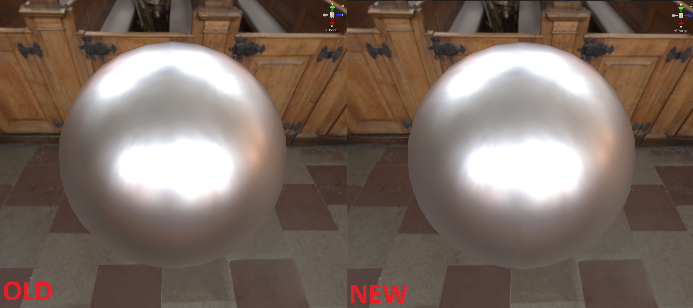
Finally, does the new method produce superior results in practice? The only difference is the weighting function, which, in Brian’s case, is further approximated by the following expression:
$$ W = FG \approx \langle n,l \rangle $$
I did some testing, and the results are pretty similar. You may notice a slight difference in saturation at the bottom of the sphere, but the original approximation is still very good, especially considering the cost.
It is possible to further improve the quality of the results by pre-filtering using MIS, or performing more intelligent filtering of the pre-filtered cubemap at runtime. But that is another story for another time.
Acknowledgments
I would like to thank Brian Karis for reviewing this blog post and offering thoughtful comments.