Realistic rendering at high frame rates remains at the core of real-time computer graphics. High performance and high fidelity are often at odds, requiring clever tricks and approximations to reach the desired quality bar.
One of the oldest tricks in the book is bump mapping. Introduced in 1978 by Jim Blinn, it is a simple way to add mesoscopic detail without increasing the geometric complexity of the scene. Most modern real-time renderers support a variation of this technique called normal mapping. While it’s fast and easy to use, certain operations, such as blending, are not as simple as they seem. This is where the so-called “surface gradient framework” comes into play.
The surface gradient framework is a set of tools to transform and combine normal (or bump) maps originally introduced by Morten Mikkelsen in his 2010 paper titled “Bump Mapping Unparametrized Surfaces on the GPU” , and further extended to handle triplanar mapping in his subsequent blog post. While there’s nothing wrong with these two publications, to really understand what’s going on, it really helps to also read his thesis, and at 109 pages, it’s quite a time investment.
Instead, I will attempt to give a shorter derivation, assuming no prior knowledge of the topic, starting from the the first principles. As with any derivation, the results will be theoretical in nature, and it’s important to understand the practical aspects. Your renderer probably doesn’t implement normal mapping this way (but maybe it should), your artists are probably used to the wrong but convenient way they’ve been doing it for decades, and your baking tool is trying to minimize the damage by reversing all of your hacks during the mesh generation step. Still, in my opinion, it’s important to understand the right way of doing things, so that, when necessary, you can make an informed decision to do things differently (optimize) and understand the implications of doing so.
Still with me? Let’s dive in.
Preliminaries, Part 1: Tangent Frame
We start with a 3D surface $S$. Assume that it has a unique 2D parametrization, e.i. an injective (one to one) mapping from a 2D texture coordinate to an object-space 3D coordinate:
$$ \tag{1} S(u,v) = \begin{bmatrix} x \cr y \cr z \end{bmatrix}. $$
You can think of it as a transformation from a 2D plane to a 3D surface. The injectivity requirement is differentiability in disguise, the property we will heavily lean on during the derivation.
Application of an affine transformation yields a set of transformed texture coordinates, which is something that’s often done to tile and translate the texture at runtime:
$$ \tag{2} \begin{bmatrix} s \cr t \end{bmatrix} = \begin{bmatrix} au+c \cr bv+d \end{bmatrix}. $$
In our notation, we will always use $[u,v]^{\mathrm{T}}$ for unique values and $[s,t]^{\mathrm{T}}$ for scaled-translated ones. Note that we don’t care about a particular surface parametrization: we can use UV-mapping, planar mapping, or something else entirely.
Armed with the surface parametrization, we can compute two tangent vectors at the surface point:
$$ \tag{3} T(u,v) = \frac{\partial S}{\partial u}, \quad B(u,v) = \frac{\partial S}{\partial v}. $$
These two vectors span the tangent plane, and are typically neither mutually orthogonal nor of unit length. It’s important to remember that they depend on the surface parametrization. You may be used to calling them “the tangent” and “the bitangent”, when, strictly speaking, the tangent plane contains infinitely many unique tangent vectors, and, to my knowledge, the term bitangent is only defined for curves.
We can use these two tangent vectors to compute the geometric normal of the surface. To make the normal independent from the surface parametrization, it should be normalized:
$$ \tag{4} N(u,v) = \frac{T \times B}{\Vert T \times B \Vert}. $$
This completes the tangent frame, which can be represented as a tangent-to-object-space matrix:
$$ \tag{5} M_{tangent}(u,v) = [T | B | N]. $$
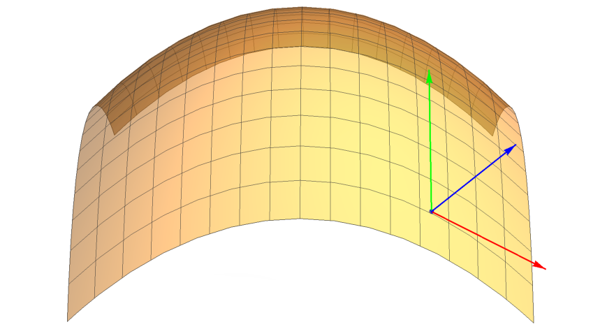
T, B and N vectors of a quadric shown in red, green and blue, respectively.
We will need the inverse of the matrix going forward:
$$ \tag{6} \begin{aligned} (M_{tangent}^{-1}(u,v))^{\mathrm{T}} = \frac{\mathrm{cof}(M_{tangent})}{\mathrm{det}(M_{tangent})} &= \frac{[B \times N | N \times T | T \times B]}{\langle T \times B, N \rangle} \cr &= \Bigg[\frac{B \times N}{\langle T \times B, N \rangle} \Bigg| \frac{N \times T}{\langle T \times B, N \rangle} \Bigg| N\Bigg]. \end{aligned} $$
In the formula above, $\mathrm{det}(M)$ is the determinant, and $\mathrm{cof}(M)$ is the cofactor matrix.
It’s important to note that, in practice, the surface parametrization used to derive the normal may be different from the texture coordinate parametrization. This means that it’s possible to encounter a mesh with vertex normals $N$ pointing in the direction opposite from $(T \times B)$. Of course, we always want to use the forward-facing normal $N$. Luckily, the math is on our side, and using the full matrix inversion procedure as described above works in all cases. More details about surface re-parametrization can be found in Morten’s thesis (see Section 2.4).
If strict compliance with the MikkT space is desired (to exactly match the assumptions of the normal map baking tool, for instance), the inverse-transpose should be replaced with the unmodified $[T | B | N]$ matrix, where $B = N \times T$ is computed either in the vertex or the pixel shader.
Preliminaries, Part 2: Height Maps and Volumes
The simplest representation of a tangent-space normal (or bump) map is the height map $z = h(s,t)$. A height map $ h(s,t) $ is a 2D subset (slice) of a 3D height volume $ h(s,t,r) $, where we use the $ r $ coordinate for the third dimension. Given a height volume, each location in space corresponds to a height (or scalar displacement) value. It’s possible define a height volume using a noise function, or by combining several height maps in a certain way (as we will see later).
A height volume is a scalar field. The gradient of a scalar field is a vector field. For a height volume, the volume gradient is a vector which points in the direction of the greatest height increase rate, with the magnitude corresponding to this rate:
$$ \tag{7} \nabla h(s,t,r) = \frac{\partial h}{\partial s} I + \frac{\partial h}{\partial t} J + \frac{\partial h}{\partial r} K = \begin{bmatrix} \partial h / \partial s \cr \partial h / \partial t \cr \partial h / \partial r \end{bmatrix}, $$
where $\lbrace I,J,K \rbrace$ is the orthonormal set of basis vectors that form the frame of reference of the height volume.
There are two equivalent ways to compute the volume gradient for a height map: one is to realize that the rate at which the scalar field changes along the third axis is zero (consider extending the height map to three dimensions by infinite replication/stacking), and the other one is to project the volume gradient onto the base plane along its normal:
$$ \tag{8} \gamma(s,t) = \frac{\partial h}{\partial s} I + \frac{\partial h}{\partial t} J = \nabla h - \langle \nabla h, K \rangle K. $$
We will refer to $ \gamma $ as the projected gradient. It is the fundamental quantity which makes bump mapping with both height maps and height volumes possible. For a height map, you can also interpret it as the height map gradient, which means that the height map gradient can be obtained by projecting the volume gradient along the normal.
Geometrically, a height map defines an implicit surface of the form:
$$ \tag{9} f(x,y,z) = z - h(x,y) = 0. $$
The upward-facing direction of the height map normal is given by the gradient of the implicit surface:
$$ \tag{10} G(x,y,z) = \nabla f(x,y,z) = \frac{\partial f}{\partial x} I + \frac{\partial f}{\partial y} J + \frac{\partial f}{\partial z} K, $$
Substitution of the height map equation readily yields the following expression:
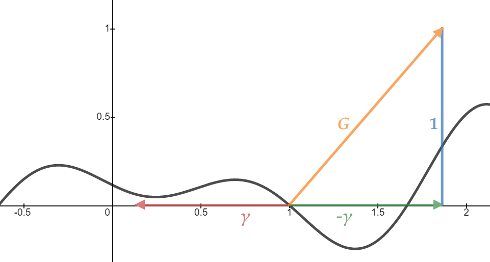
$$ \tag{11} G(s,t) = - \frac{\partial h}{\partial s} I - \frac{\partial h}{\partial t} J + K = \begin{bmatrix} -\partial h / \partial s \cr -\partial h / \partial t \cr 1 \end{bmatrix}, $$
$$ \tag{12} G(s,t) = K - \gamma. $$
We will refer to $G$ as the implicit gradient. Note that $\langle G, K \rangle$ is always 1.
It’s convenient to get the re-parametrization induced by transformed texture coordinates out of the way:
$$ \tag{13} G(u,v) = \begin{bmatrix} -\partial h / \partial s \cdot \partial s / \partial u \cr -\partial h / \partial t \cdot \partial t / \partial v \cr 1 \end{bmatrix} = \begin{bmatrix} -a \cdot \partial h / \partial s \cr -b \cdot \partial h / \partial t \cr 1 \end{bmatrix}. $$
This simply means that we need to rescale the slopes in order to adjust the displacements as we tile the texture.
For completeness, we can convert a tangent-space (height map) normal $ N_{t} = [n_{t,1}, n_{t,2}, n_{t,3}]^{\mathrm{T}} $ into the slope (gradient) form in the following way:
$$ \tag{14} G(s,t) = \begin{bmatrix} -\partial h / \partial s \cr -\partial h / \partial t \cr 1 \end{bmatrix} = \frac{N_{t}}{n_{t,3}}, $$
$$ \tag{15} G(u,v) = \begin{bmatrix} -a \cdot \partial h / \partial s \cr -b \cdot \partial h / \partial t \cr 1 \end{bmatrix} = \begin{bmatrix} -a \cdot n_{t,1} / n_{t,3} \cr -b \cdot n_{t,2} / n_{t,3} \cr 1 \end{bmatrix} = M_{tile} \frac{N_{t}}{n_{t,3}}. $$
To perturb the surface using the height map, we need to perform a change of basis from the orthonormal tangent-space set $\lbrace I,J,K \rbrace$ to our previously defined object-space set $\lbrace T,B,N \rbrace$. Doing this correctly is slightly more involved than it may seem at first glance.
Preliminaries, Part 3: Wrinkled Surfaces
The original formulation of bump mapping defines a height-mapped surface by applying a perturbation along the normal of the original surface.
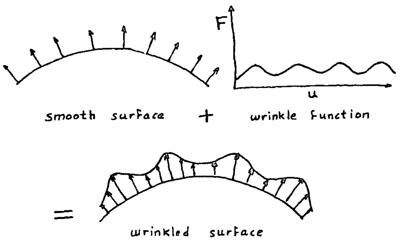
Bump mapping as depicted by Jim Blinn in his original paper.
Note that this is the right place to apply the object’s scale matrix $ M_{scale} $, as it should affect the displacements (ultimately, by scaling the slopes):
$$ \tag{16} P(u, v) = M_{scale} \Big( S(u, v) + h(u, v) N(u, v) \Big). $$
Just as we did before, we can take derivatives of this equation to compute the perturbed normal.
$$ \tag{17} T_p(u,v) = \frac{\partial P}{\partial u} = M_{scale}(T + \frac{\partial h}{\partial u} N + h \frac{\partial N}{\partial u}) \approx M_{scale}(T + \frac{\partial h}{\partial u} N), $$ $$ \tag{18} B_p(u,v) = \frac{\partial P}{\partial v} = M_{scale}(B + \frac{\partial h}{\partial v} N + h \frac{\partial N}{\partial v}) \approx M_{scale}(B + \frac{\partial h}{\partial v} N). $$
Jim claims that for small displacements and moderately curved surfaces, partial derivatives $ \partial N / \partial u $ and $ \partial N / \partial v $ are negligibly small and can be set to 0. For those interested, Morten verifies the validity of this approximation in his thesis (see Section 2.6).
We can compute the perturbed normal by taking the cross product. Just as before, we replace normalization in the denominator with the scalar triple product to avoid flipped normals:
$$ \tag{19} N_p(u,v) = \frac{T_p \times B_p}{\langle T_p \times B_p, N \rangle} \approx \frac{1}{\langle T_p \times B_p, N \rangle} \Big((M_{scale}(T + \frac{\partial h}{\partial u} N)) \times ( M_{scale}(B + \frac{\partial h}{\partial v} N)) \Big). $$
We can move the matrix outside of the brackets with the help of the following identity:
$$ \tag{20} (MA) \times (MB) = (\mathrm{det}(M))(M^{-1})^{\mathrm{T}}(A \times B) = (\mathrm{cof}(M)) (A \times B), $$
where $\mathrm{cof}(M)$ is the cofactor matrix.
$$ \tag{21} N_p(u,v) \approx \frac{\mathrm{cof}(M_{scale})}{\langle T_p \times B_p, N \rangle} \Big((T + \frac{\partial h}{\partial u} N) \times (B + \frac{\partial h}{\partial v} N)\Big). $$
Alternatively, the object scale can be incorporated directly into the $[T | B | N]$ matrix (by rescaling all three basis vectors in Equations 17 and 18).
It’s instructive to expand the cross product:
$$ \tag{22} N_p(u,v) \approx \frac{\mathrm{cof}(M_{scale})}{\langle T_p \times B_p, N \rangle} \Big((T \times B) + \frac{\partial h}{\partial u} (N \times B) + \frac{\partial h}{\partial v} (T \times N) + \frac{\partial h}{\partial u} \frac{\partial h}{\partial v} (N \times N)\Big). $$
The last term vanishes because the value of the cross product is a zero vector:
$$ \tag{23} N_p(u,v) \approx \frac{\mathrm{cof}(M_{scale})}{\langle T_p \times B_p, N \rangle} \Big((T \times B) + \frac{\partial h}{\partial u} (N \times B) + \frac{\partial h}{\partial v} (T \times N)\Big). $$
If we swap the operands of cross products, this equation will take a familiar form:
$$ \tag{24} N_p(u,v) \approx \frac{\langle T \times B, N \rangle}{\langle T_p \times B_p, N \rangle} \mathrm{cof}(M_{scale}) \frac{[B \times N | N \times T | T \times B]}{\langle T \times B, N \rangle} \begin{bmatrix} - \partial h / \partial u \cr - \partial h / \partial v \cr 1 \end{bmatrix}, $$
$$ \tag{25} N_p(u,v) \approx \frac{\langle T \times B, N \rangle}{\langle T_p \times B_p, N \rangle} \mathrm{cof}(M_{scale}) (M_{tangent}^{-1})^{\mathrm{T}}G. $$
The first term of the equation (25) can be a bit surprising. Intuitively, it accounts for the change of volume from the old to the new coordinate frame. Since it’s a non-negative scalar (negative signs of dot products, if present, cancel out), it does not modify the direction of the normal, and we can take care of it by normalizing the resulting vector.
The important part is, since normals are axial vectors (also known as antivectors), they are transformed by the inverse-transpose of the matrix. Conversely, projection of an (unscaled) object-space normal into the tangent space is performed using the transpose:
$$ \tag{26} N_o(u,v) = \frac{(M_{tangent}^{-1})^{\mathrm{T}} G}{\Vert (M_{tangent}^{-1})^{\mathrm{T}} G \Vert}, $$
$$ \tag{27} (M_{tangent})^{\mathrm{T}} N_o = \frac{(M_{tangent})^{\mathrm{T}}(M_{tangent}^{-1})^{\mathrm{T}} G}{\Vert (M_{tangent}^{-1})^{\mathrm{T}} G \Vert} = \frac{(M_{tangent}^{-1} M_{tangent})^{\mathrm{T}} G}{\Vert (M_{tangent}^{-1})^{\mathrm{T}} G \Vert} = \frac{G}{\Vert (M_{tangent}^{-1})^{\mathrm{T}} G \Vert}. $$
To transform the perturbed normal into the world space, all we have to do is rotate it. Rotation can be performed inside or outside the cofactor computation. We perform it inside for consistency.
$$ \tag{28} N_w(u,v) \approx \frac{\big( \mathrm{cof}(M_{rot} M_{scale}) (M_{tangent}^{-1})^{\mathrm{T}} \big) M_{tile} N_{t} / n_{t,3}}{\Vert \big( \mathrm{cof}(M_{rot} M_{scale}) (M_{tangent}^{-1})^{\mathrm{T}} \big) M_{tile} N_{t} / n_{t,3} \Vert}. $$
If no further modifications of the normal are desired, the matrices can be combined into a normal-tangent-to-world matrix $M_{ntw} = ((M_{rot} M_{scale} M_{tangent})^{-1})^{\mathrm{T}}$, and the division can be dropped due to subsequent normalization.
$$ \tag{29} N_w(u,v) \approx \frac{M_{ntw} M_{tile} N_{t}}{\Vert M_{ntw} M_{tile} N_{t} \Vert}. $$
If your $M_{tangent}$ transforms directly into the world space, no cofactor matrices are needed at this step. The run-time cost is thus identical to that of the traditional normal mapping.
Care must be taken when combining and interpolating these matrices, as your normal map baking tool may assume that the inverse-transpose of the tangent matrix has certain properties.
Surface Gradient Framework
The surface gradient is defined as the orthogonal projection of the volume gradient onto the tangent plane (compare to the equation (8)):
$$ \tag{30} \Gamma(u,v) = \nabla h - \langle \nabla h, N \rangle N. $$
In other words, it is the projected gradient transformed from the tangent space into the object space:
$$ \tag{31} \Gamma(u,v) = (M_{tangent}^{-1})^{\mathrm{T}} \gamma = \frac{[B \times N | N \times T] }{\langle T \times B, N \rangle} \gamma. $$
Why are these two formulas equivalent? We can use the definition of the directional derivative, which says that along any vector $W$ with its associated scalar parameter $w$, $\partial h / \partial w = \langle \nabla h, W \rangle$. Therefore,
$$ \tag{32} \begin{aligned} \gamma(u,v) &= (M_{tangent})^{\mathrm{T}} \Gamma \cr &= [T | B | N]^{\mathrm{T}} (\nabla h - \langle \nabla h, N \rangle N) \cr &= \begin{bmatrix} \partial h / \partial u \cr \partial h / \partial v \cr \langle \nabla h, N \rangle \end{bmatrix} - \begin{bmatrix} 0 \cr 0 \cr \langle \nabla h, N \rangle \end{bmatrix} = \begin{bmatrix} \partial h / \partial u \cr \partial h / \partial v \cr 0 \end{bmatrix}. \end{aligned} $$
By definition, the surface gradient is a vector in the tangent plane with the direction pointing up along the steepest slope and with the magnitude of the rate at which height increases in that direction.
Given the surface gradient, it’s easy to obtain (“resolve”) the perturbed normal:
$$ \tag{33} N_p(u,v) = \frac{(\mathrm{cof}(M_{scale}))(N - \Gamma)}{\Vert (\mathrm{cof}(M_{scale}))(N - \Gamma) \Vert}. $$
(If both the normal and the surface gradient are in the world space, the cofactor has already been applied.)
Why is it useful? Since it’s just a matrix transformation, the surface gradient is a linear operator, which, combined with the fact that the derivative is a linear operator as well, makes many common operations straightforward. Additionally, the surface gradient, like the surface normal, is independent from the surface parametrization. And finally, the surface gradient is compact, since we do not need to retain the entire tangent frame.
1. Rescaling the Height Map
Want to flatten the normal map, or make it more bumpy? Simply rescale the surface gradient:
$$ \tag{34} \alpha \Gamma(u,v) = (M_{tangent}^{-1})^{\mathrm{T}} \Big[ \frac{\partial}{\partial u} (\alpha h), \frac{\partial}{\partial v} (\alpha h), 0 \Big]^{\mathrm{T}}. $$
2. Combining Height Maps
Due to linearity, combining height maps is straightforward:
$$ \tag{35} \alpha \Gamma_{1}(u,v) + \beta \Gamma_{2}(u,v) = (M_{tangent}^{-1})^{\mathrm{T}} \Big[ \frac{\partial}{\partial u} (\alpha h_1 + \beta h_2) , \frac{\partial}{\partial v}(\alpha h_1 + \beta h_2), 0 \Big]^{\mathrm{T}}. $$
Clearly, linear blends of surface gradients are more meaningful than blends of normals themselves.
3. Object-Space Normals
Object-space normals are considered already perturbed, e.i. they do not depend on the normal of the surface. Nevertheless, it’s convenient to process them within the same framework. It’s worth keeping in mind that object-space normals retrieved from a texture should be affected by the object’s scale:
$$ \tag{36} N_p(u,v) = \frac{(\mathrm{cof}(M_{scale})) N_o}{ \Vert (\mathrm{cof}(M_{scale})) N_o \Vert }, $$
$$ \tag{37} N_o(u,v) = \frac{G_o}{ \Vert G_o \Vert } = \frac{N - \Gamma}{ \Vert N - \Gamma \Vert }. $$
It’s interesting to compare the last equation with the equation (12), and to see that they indeed match (up to the normalization factor).
While we can solve this equation for $\Gamma$ by projecting the object-space normal onto the tangent plane using the equations (27) and (31), it’s more efficient to find the solution geometrically:
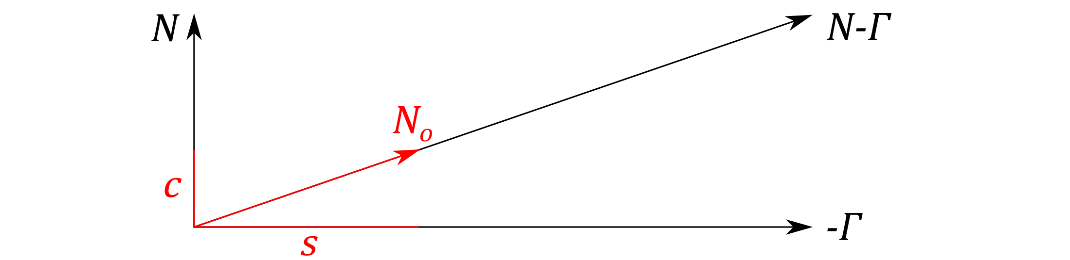
Surface gradient and the object-space normal.
$$ \tag{38} \Gamma(u,v) = N - (N - \Gamma) = N - G_o = N -\frac{N_o}{\langle N_o, N \rangle}. $$
This formula rescales the normal to obtain the corresponding implicit gradient which satisfied the condition $\langle N,G \rangle = 1$. It produces correct results even for negative values of the dot product, as well as non-unit normals $N_o$. In fact, normals can be in any space, as long as both $N$ and $N_o$ are represented with respect to the same frame of reference. Since we only deal with normals and the surface gradient, this formulation is also independent from the surface parametrization – the way we compute the texture coordinates does not matter.
4. Planar Mapping
One of the alternatives to UV-mapping is to obtain texture coordinates by projecting the surface onto a plane. Typically, the normals are stored either in the object space or in the tangent space.
The solution for the already perturbed (e.g. object-space) normals is given in the previous section. In this section, let’s find the solution for tangent-space normals.
Without loss of generality, let’s consider the X-Y plane for planar mapping. Our surface $S$ then becomes a height map w.r.t. this plane (we assume that this is a suitable parametrization for the particular surface):
$$ \tag{39} z = h(x, y), $$ $$ \tag{40} \begin{bmatrix} u \cr v \end{bmatrix} = \begin{bmatrix} x \cr y \end{bmatrix}. $$
Let’s complete the tangent frame for the new surface parametrization:
$$ \tag{41} T(u,v) = \frac{\partial S}{\partial u} = \Big[ 1, 0, \frac{\partial z}{\partial u} \Big]^{\mathrm{T}}, \quad B(u,v) = \frac{\partial S}{\partial v} = \Big[ 0, 1, \frac{\partial z}{\partial v} \Big]^{\mathrm{T}}. $$
Recall the equation (14) which relates the implicit gradient and the height map normal (which, in our interpretation, is the surface normal). We can use it to compute the values of partial derivatives:
$$ \tag{42} T(u,v) = \Big[ 1, 0, -\frac{n_{x}}{n_{z}} \Big]^{\mathrm{T}}, \quad B(u,v) = \Big[ 0, 1, -\frac{n_{y}}{n_{z}} \Big]^{\mathrm{T}}. $$
This completes the TBN for the new surface parametrization, and we can now use the equation (31) to compute the surface gradient:
$$ \tag{43} \Gamma(u,v) = \frac{1}{(n_x^2 + n_y^2 + n_z^2) / n_z} \begin{bmatrix} n_y^2/n_z+n_z & -n_x n_y/n_z \cr -n_x n_y/n_z & n_x^2/n_z+n_z \cr -n_x & -n_y \end{bmatrix} \gamma, $$
$$ \tag{44} \Gamma(u,v) = \begin{bmatrix} n_y^2+n_z^2 & -n_x n_y \cr -n_x n_y & n_x^2+n_z^2 \cr -n_x n_z & -n_y n_z \end{bmatrix} \gamma = \begin{bmatrix} 1 - n_x^2 & -n_x n_y \cr -n_x n_y & 1 - n_y^2 \cr -n_x n_z & -n_y n_z \end{bmatrix} \gamma. $$
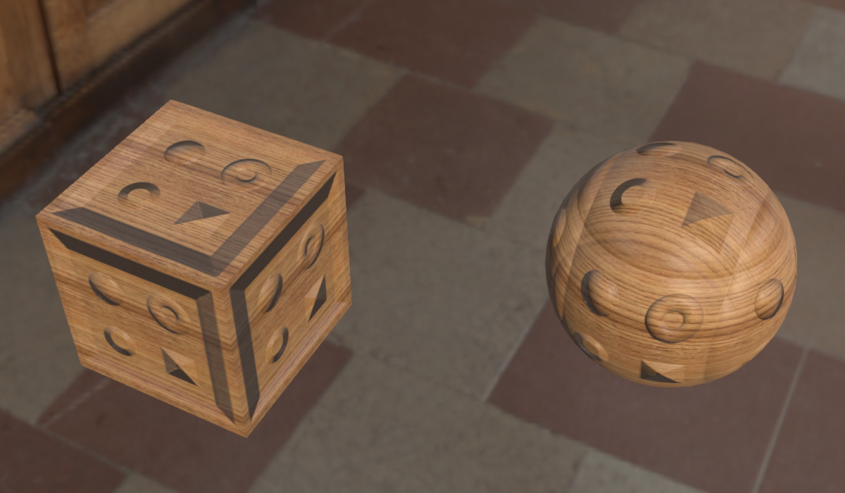
5. Tri-Planar Mapping
Tri-planar mapping is an efficient alternative to storing already perturbed normals in a cube map, or using an octahedral or lat-long projection. Instead, the same 2D texture can be reused (up to) three times for X-Y, Y-Z and Z-X planes (of course, nothing prevents us from using 3 different textures at the cost of a larger memory footprint). You can think of it as a cube map with all 6 faces of the cube using the same planar map.
The same normal map spaces supported by planar mapping are supported here. In fact, the math is almost exactly the same - the only difference is that we have to do it (up to) three times, and blend the results using the weighting function which depends on the direction of the surface normal.
But how do we blend the resulting normals? If we convert them into the surface gradient form, linear blending becomes meaningful. For object-space normals, all we have to do is blend three surface gradients (one per plane) computed using the equation (38):
$$ \tag{45} \Gamma(x,y,z) = N - w(n_x,n_y) \frac{N_1}{\langle N_1, N \rangle} - w(n_y,n_z) \frac{N_2}{\langle N_2, N \rangle} - w(n_z,n_x) \frac{N_3}{\langle N_3, N \rangle}, $$
where $w$ is the weighting function, and the normals of X-Y, Y-Z and Z-X planes are labelled as $N_1$, $N_2$ and $N_3$, respectively.
To support tangent-space normal maps, we can also blend three surface gradients obtained using the math from the previous section. However, there’s a more efficient solution presented by Morten in his blog post.
Imagine a height volume defined using three height maps (recall the infinite replication/stacking analogy) as follows:
$$ \tag{46} h(x,y,z) = w(n_x,n_y) h_z(x,y) + w(n_y,n_z) h_x(y,z) + w(n_z,n_x) h_y(z,x), $$
where $w$ is the weighting function. Let’s compute the volume gradient:
$$ \tag{47} \begin{aligned} \nabla h(x,y,z) &= \frac{\partial h}{\partial x} X + \frac{\partial h}{\partial y} Y + \frac{\partial h}{\partial z} K \cr &= X \frac{\partial}{\partial x} (w(n_x,n_y) h_z(x,y) + w(n_z,n_x) h_y(z,x)) \cr &+ Y \frac{\partial}{\partial y} (w(n_x,n_y) h_z(x,y) + w(n_y,n_z) h_x(y,z)) \cr &+ Z \frac{\partial}{\partial z} (w(n_y,n_z) h_x(y,z) + w(n_z,n_x) h_y(z,x)). \end{aligned} $$
The expression is a little complicated, particularly because both the height and the weighting functions depend on the position, so we would need to apply the product rule in order to compute the derivative. Instead, Morten employs a simplification (identical to the one in the “Wrinkled Surfaces” section), assuming that the normals and, as a result, the weights vary slowly w.r.t. the position:
$$ \tag{48} \frac{\partial N}{\partial x} = \frac{\partial N}{\partial y} = \frac{\partial N}{\partial z} = 0. $$
It considerably simplifies the initial equation:
$$ \tag{49} \begin{aligned} \nabla h(x,y,z) &= X \Big(w(n_x,n_y) \frac{\partial h_z(x,y)}{\partial x} + w(n_z,n_x) \frac{\partial h_y(z,x)}{\partial x} \Big) \cr &+ Y \Big(w(n_x,n_y) \frac{\partial h_z(x,y)}{\partial y} + w(n_y,n_z) \frac{\partial h_x(y,z)}{\partial y} \Big) \cr &+ Z \Big(w(n_y,n_z) \frac{\partial h_x(y,z)}{\partial z} + w(n_z,n_x) \frac{\partial h_y(z,x)}{\partial z} \Big). \end{aligned} $$
To verify correctness, let’s compare it with the equation (44) for the X-Y plane. We assume that the only non-zero weight is $w(n_x,n_y) = 1$, and compute the surface gradient using the equation (30):
$$ \tag{50} \begin{aligned} \Gamma(x,y) &= \nabla h - \langle \nabla h, N \rangle N \cr &= \Big[ \frac{\partial h}{\partial x}, \frac{\partial h}{\partial y}, 0 \Big]^{\mathrm{T}} - \Big \langle \Big[ \frac{\partial h}{\partial x}, \frac{\partial h}{\partial y}, 0 \Big]^{\mathrm{T}}, N \Big \rangle N \cr &= \Big[ \frac{\partial h}{\partial x}, \frac{\partial h}{\partial y}, 0 \Big]^{\mathrm{T}} - \frac{\partial h}{\partial x} n_x N - \frac{\partial h}{\partial y} n_y N \cr &= \begin{bmatrix} 1 - n_x^2 & -n_x n_y \cr -n_x n_y & 1 - n_y^2 \cr -n_x n_z & -n_y n_z \end{bmatrix} \begin{bmatrix} \partial h / \partial x \cr \partial h / \partial y \end{bmatrix}. \end{aligned} $$
If we recall that our planar mapping example assumes that $ [ u,v ]^{\mathrm{T}} = [ x,y ]^{\mathrm{T}} $, we can see that the two expressions are indeed identical.
Conclusion
The surface gradient framework offers powerful tools for processing different representations of bump maps: height maps, height volumes, normal maps, in any space or frame of reference. At its core is the original bump mapping algorithm of Jim Blinn, which stands the test of time.
If you want to learn more, I encourage you to check out the papers referenced in the introduction. They contain plenty of interesting details which will help you master of the intricate subject of bump mapping.
Acknowledgments
I would like to thank Jim Blinn and Brian Karis for reviewing this blog post and offering thoughtful comments. Special thanks to Morten Mikkelsen for answering my questions.