Sampling Burley's Normalized Diffusion Profiles

2019-12-16

A couple of years ago, I worked on an implementation of Burley’s Normalized Diffusion (a.k.a. Disney SSS). The original paper claims that the CDF is not analytically invertible. I have great respect for both authors, Brent Burley and Per Christensen, so I haven’t questioned their claim for a second. Turns out, “Question Everything” is probably a better mindset.

I’ve been recently alerted by @stirners_ghost on Twitter (thank you!) that the CDF is, in fact, analytically invertible. Moreover, the inversion process is almost trivial, as I will demonstrate below.

The diffusion model is radially symmetric, and is defined as

$$ \tag{1} R(r) = \frac{A s}{8 \pi r} \Big( e^{-s r} + e^{-s r / 3} \Big). $$

To find the corresponding PDF, it must be normalized:

$$ \tag{2} \int_{-\infty}^{\infty} \int_{-\infty}^{\infty} \frac{R(\sqrt{x^2+y^2})}{A} dx dy = \int_{0}^{2 \pi} \int_{0}^{\infty} \frac{R(r)}{A} r dr d\theta = \int_{0}^{2 \pi} \int_{0}^{\infty} p_r(r, \theta) dr d\theta = 1. $$

Therefore, in polar coordinates, the PDF is given as

$$ \tag{3} p_r(r, \theta) = \frac{R(r)}{A} r = \frac{s}{8 \pi} \Big( e^{-s r} + e^{-s r / 3} \Big). $$

The marginal CDF is then

$$ \tag{4} P(r) = \int_{0}^{2 \pi} \int_{0}^{r} p_r(z, \theta) dz d\theta = 1 - \frac{1}{4} e^{-s r} - \frac{3}{4} e^{-s r / 3}. $$

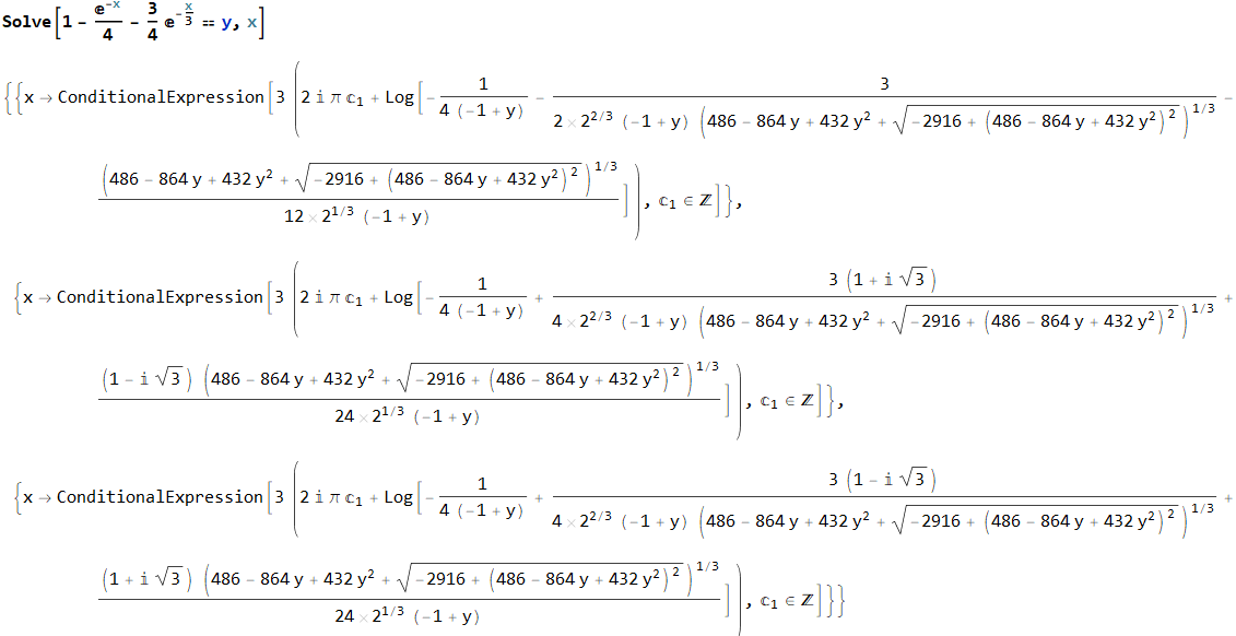
Let us define $x = s r$. If we ask Mathematica to solve $y = P(x)$ for $x$ in order to obtain the inverse $x = P^{-1}(y)$, we get a somewhat terrifying (but, of course, correct) output:

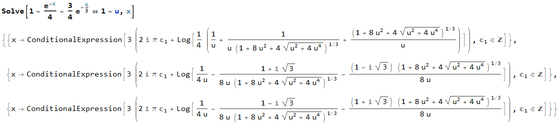
The trick is to solve $P(x) = 1 - u$ instead (where $u = 1 - P(x)$ is the complementary CDF):

To get rid of the imaginary part, we can set the free constant $c_{1} = 0$, which results in the following inverse:

$$ \tag{5} x = s r = 3 \log{\Bigg(\frac{1 + G(u)^{-1/3} + G(u)^{1/3}}{4 u} \Bigg)}, $$

where

$$ \tag{6} G(u) = 1 + 4 u \Big( 2 u + \sqrt{1 + 4 u^2} \Big). $$

We can verify that it works by feeding the complementary CDF with its inverse.

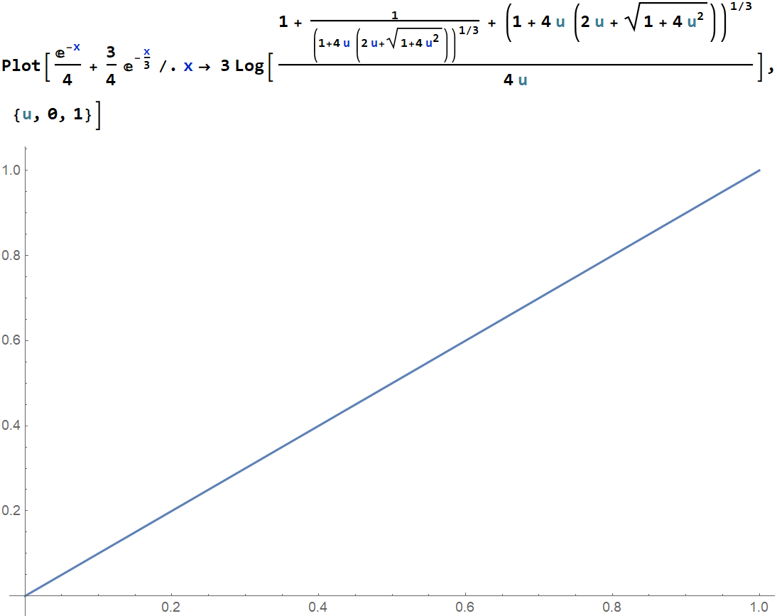
For importance sampling, we can uniformly sample either the complementary or the regular CDF - it makes no difference $($except for reversing the order of samples, s.t. $x(0) = \infty$ and $x(1) = 0 )$.

An optimized implementation is listed below.

// Performs sampling of a Normalized Burley diffusion profile in polar coordinates.
// 'u' is the random number (the value of the CDF): [0, 1).
// rcp(s) = 1 / ShapeParam = ScatteringDistance.
// 'r' is the sampled radial distance, s.t. (u = 0 -> r = 0) and (u = 1 -> r = Inf).
// rcp(Pdf) is the reciprocal of the corresponding PDF value.
void SampleBurleyDiffusionProfile(float u, float rcpS, out float r, out float rcpPdf)
{
    u = 1 - u; // Convert CDF to CCDF; the resulting value of (u != 0)

    float g = 1 + (4 * u) * (2 * u + sqrt(1 + (4 * u) * u));
    float n = exp2(log2(g) * (-1.0/3.0));                    // g^(-1/3)
    float p = (g * n) * n;                                   // g^(+1/3)
    float c = 1 + p + n;                                     // 1 + g^(+1/3) + g^(-1/3)
    float x = (3 / LOG2_E) * log2(c * rcp(4 * u));           // 3 * Log[c / (4 * u)]

    // x      = s * r
    // exp_13 = Exp[-x/3] = Exp[-1/3 * 3 * Log[c / (4 * u)]]
    // exp_13 = Exp[-Log[c / (4 * u)]] = (4 * u) / c
    // exp_1  = Exp[-x] = exp_13 * exp_13 * exp_13
    // expSum = exp_1 + exp_13 = exp_13 * (1 + exp_13 * exp_13)
    // rcpExp = rcp(expSum) = c^3 / ((4 * u) * (c^2 + 16 * u^2))
    float rcpExp = ((c * c) * c) * rcp((4 * u) * ((c * c) + (4 * u) * (4 * u)));

    r      = x * rcpS;
    rcpPdf = (8 * PI * rcpS) * rcpExp; // (8 * Pi) / s / (Exp[-s * r / 3] + Exp[-s * r])
}

Acknowledgments

I would like to thank @stirners_ghost for informing me that the CDF is invertible, and Brent Burley for spotting a missing minus sign in the derivation.

Acknowledgments

Contents