I have previously covered the basics of the volume scattering process. It models the macroscopic interaction of light and matter, with the latter represented as a distribution of small particles. Fundamentally, the volume scattering process arises from the microscopic interaction of light with individual atoms, and is typically described using Maxwell’s electromagnetic theory. It is the domain of optics, and, in my experience, the connection with the radiative transfer equation is neither apparent nor easy to find. The purpose of this blog post is to familiarize the reader with domain-specific terms and ease the adoption of formulas found in the optics literature.
Radiometry Crash Course
Imagine a light sensor (or a photon detector, with each photon carrying $h \nu$ joules of energy) with the surface area $\sigma_n$ and the surface normal1 $\bm{n}$. We would like to measure the amount of radiant energy $Q_n$ absorbed by (or passing through) the sensor during the period of time $t$. This can be done in several different ways, depending on the parametrization of the incident radiation.
If the spectral flux $\Phi_n$ in the frequency interval $d\nu$ reaches the sensor,
$$ \tag{1} dQ_n = \Phi_n d\nu dt. $$
The flux is a very coarse quantity in the sense that it does not tell us where the radiation is coming from and to what degree the different parts of the sensor are affected.
In case the flux density on the surface is known, it is given by the spectral irradiance $E_n$:
$$ \tag{2} dQ_n = E_n d\sigma_n d\nu dt. $$
If we can only determine the directional characteristics of the flux, it can be represented using the spectral intensity $I_i$:
$$ \tag{3} dQ_n = I_i d\Omega_i d\nu dt, $$
where $d\Omega_i$ is the solid angle measure associated with the incident direction $\bm{i}$. Note that the left-hand side of the equation depends on the surface orientation; thus, so does the right-hand side.
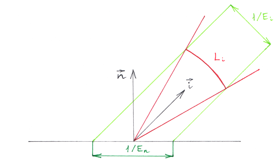
The spectral radiance $L_i$ specifies2 both the spatial and the directional densities of the flux:
$$ \tag{4} dQ_n = L_i \cos{\theta} d\Omega_i d\sigma_n d\nu dt, $$
where $\cos{\theta} = \bm{i} \cdot \bm{n}$ is the projection factor. It can be used to define the projected area measure $d\sigma_i = d\sigma_n \cos{\theta}$ $(d\sigma_n$ projected along $\bm{i})$ and the projected solid angle measure $d\Omega_n = d\Omega_i \cos{\theta}$ $(d\Omega_i$ projected along $\bm{n})$.
Unlike the projected solid angle which is measured with respect to the surface, the projected area is measured across the beam of incident radiation. Thus, so is the spectral radiance:
$$ \tag{5} dQ_n = L_i d\Omega_i d\sigma_i d\nu dt. $$
These equations show that $I_i$ and $E_n$ are orientation-dependent:
$$ \tag{6} I_i = \int_{\sigma_n \cos{\theta}} L_i d\sigma_i, \quad E_n = \int_{\Omega} \cos{\theta} L_i d\Omega_i. $$
We could address this issue by using the vector irradiance $\bm{E}$,
$$ \tag{7} E_n = \bm{n} \cdot \bm{E} = \bm{n} \cdot \int_{\Omega} \bm{i} L_i d\Omega_i = \bm{n} \cdot \int_{\Omega} \bm{i} dE_i, $$
which is defined in terms of the spectral irradiance measured across the beam (per beam):
$$ \tag{8} dE_i = \frac{dE_n}{\cos{\theta}} = L_i d\Omega_i. $$
Intensity vs irradiance.
Independence from the surface orientation coupled with invariance along the ray makes the (basic) radiance a very useful quantity for light transport applications.
In practice, most authors write Equation 4 this way:
$$ \tag{9} dQ_i = L_i \cos{\theta} d\Omega_i d\sigma d\nu dt, $$
with all the $X_n$ quantities considered incident and thus written as $X_i$. We shall adopt this convention as well.
By reciprocity, if we turn the sensor into an emitter and replace $\bm{i}$ with $\bm{o}$, the resulting equations remain valid.
For additional details, see Chapter 3 of Veach’s Ph.D. thesis and the references listed therein.
Light Scattering by a Single Particle
The interaction of light with an individual particle is quantified by the differential scattering cross section $\sigma_s’$. It is defined as the ratio of the spectral intensity3 $I_o$ scattered in the given direction $\bm{o}$ to the spectral irradiance $E_i$ incident from the direction $\bm{i}$:
$$ \tag{10} \sigma_s’(\bm{i}, \bm{o}) = \frac{d \sigma_s}{d \Omega_o} = \frac{I_o}{E_i}. $$
There is an implicit dependence on the orientation of the particle with respect to the incident wave - it comes into play if the particle is anisotropic.
We can obtain the scattering cross section $\sigma_s$ by integrating over $4 \pi$ steradians:
$$ \tag{11} \sigma_s(\bm{i}) = \int_{4 \pi} \sigma_s’ d \Omega_o = \frac{\int_{4 \pi} I_o d \Omega_o}{E_i} = \frac{\Phi_o}{E_i}. $$
In other words, it is just the ratio of the scattered spectral flux $\Phi_o$ to the incident spectral irradiance $E_i$. It has the dimensions of an area; however, it is not a geometrical area. It can be imagined as a small disk4 normal with respect to the incident beam $\bm{i}$ (don’t be confused by the subscript $s$).
The extinction cross section $\sigma_t$ relates the total spectral flux $\Phi_t$ scattered or absorbed by the particle (e.i. removed from the incident wave) to the incident spectral irradiance $E_i$:
$$ \tag{12} \sigma_t(\bm{i}) = \sigma_s + \sigma_a = \frac{\Phi_o}{E_i} + \frac{\Phi_a}{E_i} = \frac{\Phi_t}{E_i}. $$
The optical cross sections $\sigma_x$ are related to the geometrical cross section $\sigma_g$ by the efficiencies $Q_x$:
$$ \tag{13} Q_a = \frac{\sigma_a}{\sigma_g} = \frac{\Phi_a}{\Phi_i}, \qquad Q_s = \frac{\sigma_s}{\sigma_g} = \frac{\Phi_o}{\Phi_i}, \qquad Q_t = \frac{\sigma_t}{\sigma_g} = \frac{\Phi_t}{\Phi_i}. $$
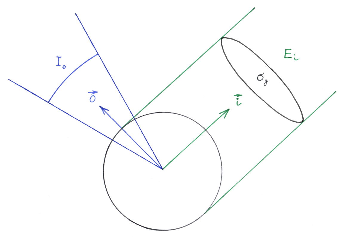
Geometrical cross section of a particle.
Note that the value of extinction efficiency can exceed 1. This phenomenon is called the extinction paradox.
The angular distribution of scattered light is described by the phase function $f_p$:
$$ \tag{14} f_p(\bm{i}, \bm{o}) = \frac{I_o}{\frac{1}{4 \pi} \int_{4 \pi} I_o d \Omega_o} = \frac{I_o}{\frac{1}{4 \pi} \Phi_o}. $$
It is the ratio of the energy per unit solid angle scattered in a given direction $\bm{o}$ to the average energy per unit solid angle scattered in all directions. Again, there is an implicit dependence on the orientation of the particle with respect to the incident wave. Note that the integral of the phase function over $4 \pi$ steradians equals $4 \pi$, which appears to be a common convention in optics.
Let us compute the product of the scattering cross section and the phase function:
$$ \tag{15} \sigma_s(\bm{i}) f_p(\bm{i}, \bm{o}) = \frac{\Phi_o}{E_i} \frac{I_o}{\frac{1}{4 \pi} \Phi_o}. $$
The spectral flux cancels out, and we find the connection with the differential scattering cross section:
$$ \tag{16} \sigma_s’(\bm{i}, \bm{o}) = \sigma_s \frac{f_p}{4 \pi}. $$
For a more elaborate derivation based on wave optics, see Chapter XIII of Born & Wolf, Principles of optics, or Chapter 2 of Mishchenko, Travis & Lacis, Scattering, Absorption, and Emission of Light by Small Particles.
Light Scattering by a Group of Particles
Let us see how we can extend this theory to scattering by $N$ particles. When an atom interacts with light, it experiences a periodic perturbation of its electron cloud, which turns it into a source of radiation. Assuming elastic scattering (ignoring the Raman effect), this radiation will have the same frequency as the incident light. Additionally, assuming that all the particles are identical (including their orientation), they will all radiate energy in exactly the same way.
The resulting electromagnetic waves will combine at the detector, potentially experiencing both constructive and destructive interference. Since all the particles are identical, the only differentiating factor is their position, which means that the scattered waves will have different phases (due to variation of distances from the particles to the detector). Making the final assumption that these particles are randomly distributed in a small region of space, we can decorrelate their phases. This results in incoherent scattering, with constructive and destructive interference canceling each other out (as we average over space and time), and it can be shown that the mean energy carried by the combined wave simply increases by a factor of $N$.
Therefore, we can rewrite Equations 10 and 16 for $N$ particles as
$$ \tag{17} I_o = N \sigma_s \frac{f_p}{4 \pi} E_i. $$
One way to see it is as if the scattering cross section increases by a factor of $N$.
“Wait a minute”, you may object. “Shouldn’t we also consider the effect of scattered waves on the particles themselves?” And, in general, indeed, we should. This is a many-body problem, and it is extremely challenging to solve exactly. In a low-density dielectric (a gas), electromagnetic interaction between the particles is typically neglected - this is sometimes referred to as the independent scattering approximation. For dense dielectrics, one way of tackling the problem is to introduce the electric polarization - induced electric dipole moment per unit volume - which can be used to approximate the local electric field.
We can extend Equation 17 to take the volume occupied by particles into account. Given a number of particles $dN$ contained within a small volume $dV$,
$$ \tag{18} \frac{dI_o}{dV} = \frac{dN}{dV} \sigma_s \frac{f_p}{4 \pi} E_i. $$
$dN / dV$ is the definition of the number density $n$, and can be used to define the scattering coefficient $\beta_s$
$$ \tag{19} \beta_s = n \sigma_s. $$
Substitution yields
$$ \tag{20} \frac{dI_o}{dV} = \beta_s \frac{f_p}{4 \pi} E_i. $$
If a distribution of (non-identical) particles is given, under the same assumptions as above, we can use its weighted average properties instead:
$$ \tag{21} \langle \beta_x \rangle = \int n(r) \sigma_x(r) dr, $$
$$ \tag{22} \langle f_p \rangle = \frac{\int n(r) \sigma_s(r) f_p(r) dr}{\int n(r) \sigma_s(r) dr}. $$
If we orient the direction of scattering along the $z$-axis, we may write
$$ \tag{23} \frac{dI_o}{d\sigma dz} = \beta_s \frac{f_p}{4 \pi} E_i. $$
The ratio of spectral intensity (normal) to the area is the definition of scattered spectral radiance $L_o$:
$$ \tag{24} \frac{dL_o}{dz} = \beta_s \frac{f_p}{4 \pi} E_i. $$
Intuitively, the “left-over” $dz$ makes sense. If we increase $dz$, the total volume increases, the density correspondingly decreases, and, since the number of particles remains constant, the amount of spectral radiance does not change.
In light transport applications, we typically deal with radiance rather than irradiance. This can be achieved by substituting5 Equation 8 and introducing an integral over $4 \pi$ steradians:
$$ \tag{25} dL_o = \int_{4 \pi} \beta_s \frac{f_p}{4 \pi} L_i d \Omega_i dz. $$
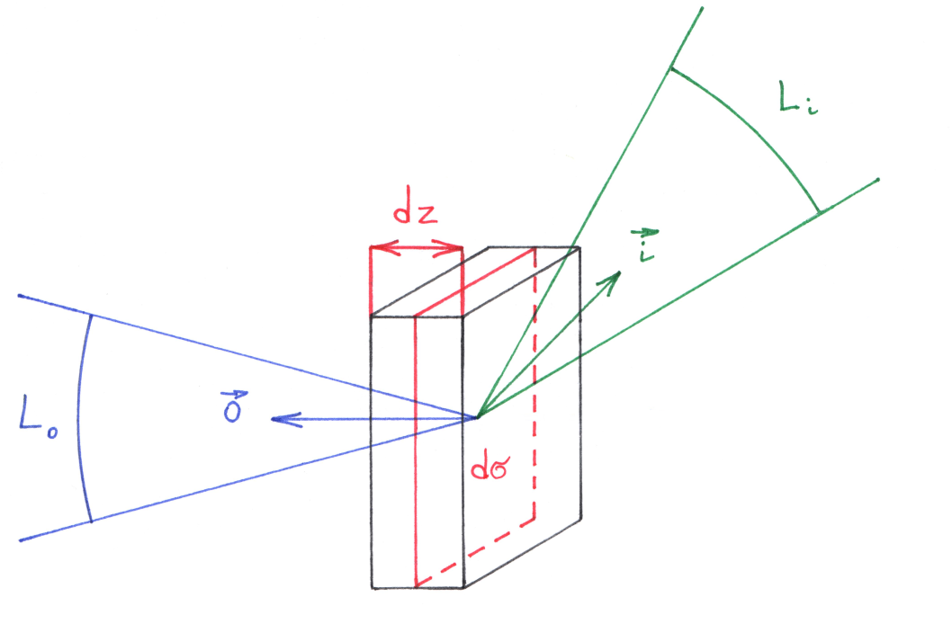
Scattering by a volume element.
Finally, we must perform line integration along the $z$-axis
$$ \tag{26} L_o = \int_{\bm{x}}^{\bm{y}} T(\bm{x}, \bm{z}) \int_{4 \pi} \beta_s \frac{f_p}{4 \pi} L_i d \Omega_i dz, $$
and add the transmittance term $T$ to account for absorption and scattering over the (non-infinitesimal) distance from the scatterer to the sensor.
By recursively defining $L = L_i = L_o$, we obtain6 the familiar radiative transfer equation.
For a derivation from the volume scattering viewpoint, see Chapter I of Chandrasekhar, Radiative transfer.
Acknowledgments
I would like to thank Eugene d’Eon for his thoughtful comments and feedback, and Don Grainger for his book and for reviewing this article.
-
If the sensor is not planar, the normal $\bm{n}$ is a function of position $\bm{x}$. However, it is simpler to think of the sensor as a manifold composed of infinitesimal rectangles. ↩︎
-
Historically, radiance was called intensity and spectral radiance was called specific intensity. Personally, I don’t find this name to be sufficiently specific. ↩︎
-
The reason we use intensity rather than radiance is that the scatterer acts as a point charge (or a point source, if you will). While the particle does have an area, its entire volume scatters light, which means that a volume (rather than an area) energy density measure would be more appropriate. ↩︎
-
The “small disk” model is convenient in problems of light scattering by spherical particles since their geometrical cross section is also a disk. In the volume scattering case, the volume element is typically a rectangular cuboid, which makes the “little square” model more appropriate for describing the cross sections. ↩︎
-
The cosine factor does not appear in the calculation because the scattering cross section is, by definition, normal to the direction of incidence. ↩︎
-
If we wish to model the refractive radiative transfer equation instead, we must remember to also account for continuous reflection/transmission as well as the associated change in the solid angle. ↩︎