High Z-buffer precision is something that we take for granted these days. Since the introduction of reversed floating-point Z-buffering (and, assuming you use the standard tricks like camera-relative transforms), most depth precision issues are a thing of the past. You ask the rasterizer to throw triangles at the screen and, almost magically, and they appear at the right place and in the right order.
There are many existing articles concerning Z-buffer precision (1, 2, 3, 4, 5, 6, 7, the last one being my favorite), as well as sections in the Real-Time Rendering and the Foundations of Game Engine Development books. So, why bother writing another one? While there is nothing wrong with the intuition and the results presented there, I find the numerical analysis part (specifically, its presentation) somewhat lacking. It is clear that “the quasi-logarithmic distribution of floating-point somewhat cancels the $1/z$ nonlinearity”, but what does that mean exactly? What is happening at the binary level? Is the resulting distribution of depth values linear? Logarithmic? Or is it something else entirely? Even after reading all these articles, I still had these nagging questions that made me feel that I had failed to achieve what Jim Blinn would call the ultimate understanding of the concept.
In short, we know that reversed Z-buffering is good, and we know why it is good; what we would like to know is what good really means. This blog post is not meant to replace the existing articles but, rather, to complement them.
With that in mind, the goals of this article are:
- Consider a typical case using actual 32-bit floating-point depth values, as well as a realistic depth range.
- Analyze numerical results and draw conclusions.
- Show all steps of the analysis in detail (get my Mathematica script here).
If that is something that interests you, please read on.
Reversed Z-Buffering Basics
We can perform a perspective transformation of a column vector representing a view-space point using the matrix
$$ \tag{1} \bm{P_r} = \begin{bmatrix} p/a & 0 & 0 & 0 \cr 0 & p & 0 & 0 \cr 0 & 0 & -n/(f-n) & f n / (f-n) \cr 0 & 0 & 1 & 0 \end{bmatrix}, $$
where $a$ is the aspect ratio of the sensor, and $n,f,p$ are the distances to the near, far, and projection planes, respectively. This particular projection matrix is symmetric, and does not have an oblique near plane; these cases are less common, and they make the analysis more complicated.
The resulting vector will have 4 components: $[x’,y’,z’,w]^{\mathrm{T}}$. We can see that the $w$ component is equal to the third coordinate of the original view-space point (the so-called “linear depth”), and we shall label it this way. We can obtain the value stored in the Z-buffer value by means of perspective division: $z=z’/w$.
Stated more precisely,
$$ \tag{2} z(w) = \frac{1}{w} \frac{f n}{f-n} - \frac{n}{f-n}. $$
Since the projection is reversed, it can be shown that $z(n)=1$ and $z(f)=0$.
Then, either by inverting the projection matrix, or solving Equation (2) for $w$, we can recover
$$ \tag{3} w(z) = \frac{f n}{n + z (f-n)}. $$
We shall examine a fairly typical open-world case of $n=0.1$ and $f=10000$ meters. First, let us plot $w$ against $z$.
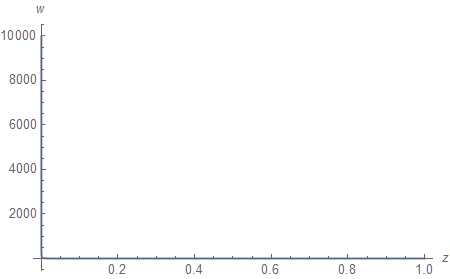
This behavior is typical for functions of $\mathrm{O}(z^{-1})$: there is a strong peak as $z \to 0$ and a long tail as $z \to \infty$.
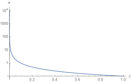
Plotting the same graph on a logarithmic scale (compare the vertical axes) allows us to take a better look:
Fixed-Point Z-Buffer
In order to become more familiar with the process of analysis, and to obtain a comparison point, let us consider a simple case of an unsigned, normalized, fixed-point Z-buffer. Assuming 24-bit binary storage $(k=24)$ that we interpret as a decimal number $d$, we can compute the depth value it represents as follows:
$$ \tag{4} \upsilon(d) = \frac{d}{2^k-1} = \frac{d}{16777215}. $$
Plugging $\upsilon$ instead of $z$ into Equation (3) allows us to map the values stored within the Z-buffer to the original linear depth values they represent.
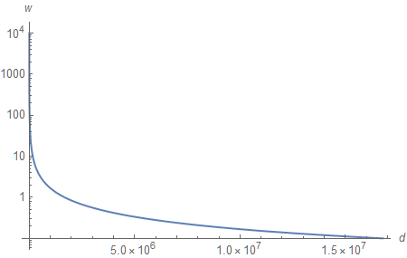
Since we obtain $\upsilon$ by linearly transforming (scaling) $d$, the graph looks identical to the one from the previous section. Unfortunately, it means that over 90% of the values of $d$ are used for objects less than 1 meter away from the viewer.
Since we are interested in precision of the Z-buffer, we should find a way to plot its resolution. By resolution, we mean the smallest positive linear depth difference (smaller is better) that results in a different binary value of $z$ (some may consider this number a “reciprocal of resolution”; the definition and the naming are both deliberate to simplify discussion and plotting). In other words, for a certain decimal number $d$, it is the absolute difference $\Delta w$ between the linear depth value $d$ corresponds to and the linear depth value of its immediate neighbor.
Mathematically, for a continuous function, we can obtain the desired graph by plotting the absolute value of the derivative
$$ \tag{5} \Delta w \approx \Bigg\lvert \frac{\partial w \big( \upsilon(d) \big)}{\partial d} \Bigg\rvert. $$
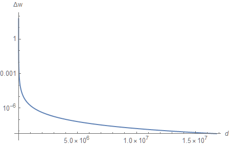
The graph looks remarkably similar to the previous one (except for the scale). But, in fact, it is not - the derivative of $\mathrm{O}(z^{-1})$ is $\mathrm{O}(z^{-2})$. The logarithmic scale we use for plotting can be a little misleading.
We can make the resulting graph easier to read by converting the $d$-axis to the $w$-axis. Intuitively, what we want to do is to replace the horizontal axis of the current graph with the vertical axis of the previous one. We can do that by (literally) converting the graph into a large list of pairs $\lbrace d, \Delta w \rbrace$, and then, for each one, replacing the number $d$ with the value of $w$ it corresponds to, and plotting these pairs as points.
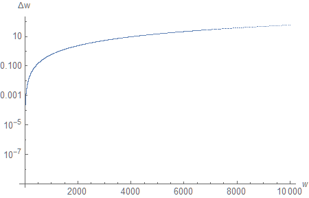
Because of the Z-reversal, the new graph appears transposed. But now it is more clear that, for instance, the depth resolution falls below 1 meter at distances exceeding 1000 meters.
Floating-Point Z-Buffer
We proceed in a similar fashion by defining a function that interprets a decimal number as a binary representation of a floating-point number. In lieu of reinterpret_cast, this function can be defined as
$$ \tag{6} \phi(d) = s_{\phi} (1 + t_{\phi}) 2^{e_{\phi}-b}, $$
where
$$ \tag{7} \begin{aligned} s_{\phi}(d) &= 1 - 2 \left\lfloor 2^{1-k} d \right\rfloor, \cr e_{\phi}(d) &= \left\lfloor 2^{-t} d \right\rfloor - 2^{k-t-1} \left\lfloor 2^{1-k} d \right\rfloor, \cr t_{\phi}(d) &= \sum_{i=0}^{t-1} 2^{i-t} \left(\left\lfloor 2^{-i} d \right\rfloor -2 \left\lfloor 2^{-i-1} d \right\rfloor \right), \end{aligned} $$
are the sign, the biased exponent, and the trailing significand, respectively. The IEEE standard defines $k=32,t=23,b=127$ as encoding parameters for 32-bit floating-point numbers. Additionally, we should keep in mind that the values of $z$ are restricted to the unit interval, so, assuming denormal numbers are flushed to zero, $d$ can either be zero or take on values in the range $[1 \times 2^{23}, 127 \times 2^{23}] = [8388608, 1065353216]$. That is less than a quarter of all 32-bit decimal numbers (however, it is also 63 times more values than can be stored in a 24-bit buffer). Additionally, this puts a well-defined upper bound on potential precision improvements that could result from expanding the range of values of $z$.
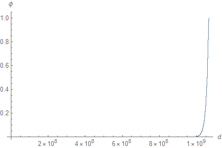
Plotting Equation 6 as a function of $d$ reveals that the first billion values of $\phi$ are very small.
The quasi-exponential nature of the function can be clearly observed if we zoom in near $\phi = 1$.
Zooming in some more, we can see that the function we defined is, in fact, constant between subsequent values of $d$ (one can make the case that it should be constant between midpoints, but we will ignore rounding subtleties in this analysis).
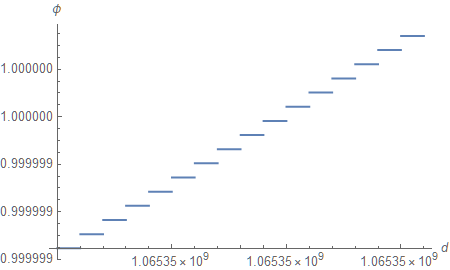
This is the limit of floating-point precision. All values that fall in-between must be rounded to machine-representable ones.
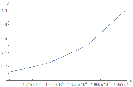
Substitution of $\phi$ for $z$ in Equation (3) allows us to plot linear depth against $d$.
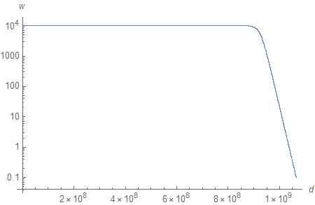
You may find the graph surprising (I certainly did). We only see an exponential distribution of $w$ appear after around 900 million values. To give you some idea of the numbers on the horizontal line, $\phi(7 \times 10^8) \approx 8.22242 \times 10^{-14}$ and $w \big(\phi(7 \times 10^8)\big) \approx 9999.9999$. If we consider only the last 10% of the values of $d$, they cover 90% of the viewing range. So, in fact, the actual useful range of decimal values is even smaller than originally anticipated. (“It may be worth pointing out that the long horizontal segment on this graph corresponds to the “long tail” of exceedingly small floating-point values (e.g. 2⁻²⁰ down to 2⁻¹²⁷). Consulting Equation (3), we can see that when we have a finite far plane, then whenever z ≪ n/f in magnitude, we will have w ≈ f. Here, n/f = 10⁻⁵ so any z values from 10⁻⁶ or so on down will be crushed against the far plane and basically useless. Setting an infinite far plane alleviates this problem.” - Nathan Reed)
What about precision, then? Since ${\phi}$ is constant between (and discontinuous at) subsequent decimal values, we cannot really use standard methods of real analysis such as taking the derivative. But, since we are just interested in the difference between linear depth values for successive decimal numbers, we can approximate $\partial w / \partial d$ using finite differences which operate exactly that way:
$$ \tag{8} \Delta w \approx \Bigg\lvert \frac{w \big( {\phi}(d+1) \big) - w \big( {\phi}(d-1) \big)}{2} \Bigg\rvert. $$
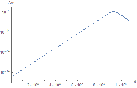
Do you recall the quasi-linear segments of ${\phi}$ we saw earlier? The derivative of a linear function is a constant, so, if you zoom in a little bit, that is exactly what you see on the left side of the graph (where $w$ is practically constant). We have an absurdly high level of precision at the far plane $(d \to 0)$, but, most importantly, the depth resolution stays fairly high throughout the whole range.
For completeness, we can zoom in near ${\phi} = 1$ again (on a linear scale to facilitate comparison).
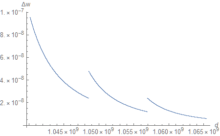
At this point $w$ is exponentially decreasing, so the interaction between $1/z$ and the quasi-exponential floating-point behavior is more complex. The gaps correspond to the endpoints of subsequent quasi-linear segments of ${\phi}.$ Admittedly, they are larger than I anticipated. If you have a theory why that is the case, please feel free to share it with the rest of the community on Twitter.
As before, we can swap the $d$-axis for the $w$-axis.
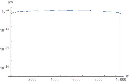
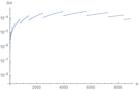
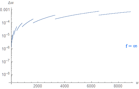
This really puts things into perspective (I encourage you to compare the graph of $\Delta w(d)$ with this one). First, we have sub-millimeter resolution across the entire depth range. More interestingly, it remains approximately constant, except for the regions located next to the near and far planes, where we allocate most of the available bits. In fact, including the far plane is skewing the graph so much that, if we only consider $n \leq w \leq 9000$ $(d > 0.9 \times 10^9)$, it paints a rather different picture:
With so much precision allocated for the region near the far plane, it is natural to wonder how the distance to the far plane affects the depth resolution. Can we push it infinitely far away “for free”?
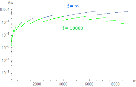
Turns out, if we do that, precision is barely affected for distances up to around 1000 meters. As we get farther away from the camera, precision no longer remains constant, and starts to drop in a linear fashion (to be more specific: precision decreases approximately linearly up to the distance of 1000 meters for both $f=10000$ and $f \to \infty$; the behavior varies past that point). We can see that if we create a plot with both axes using a logarithmic scale.
Considering the expanded viewing range, that is a perfectly reasonable trade-off.
You may wonder how it compares to a 32-bit fixed-point logarithmic depth buffer. By definition, it has constant relative precision, such that $(\Delta w)/w \in \mathrm{O}(1)$. More intuitively, $\Delta w \in \mathrm{O}(w)$, which implies that the depth resolution scales linearly with distance.
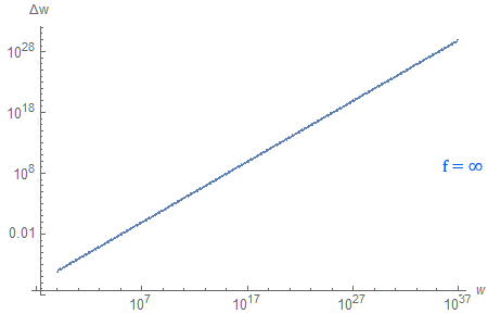
Turns out, if we plot both (using $f = 10^{37}$ to maintain the scale of the graph), they are surprisingly close.
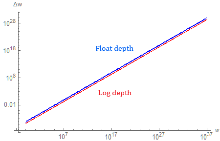
The floating-point Z-buffer is slightly behind in terms of depth resolution, which can be partially explained by the fact that it only uses around a quarter of available values of $d$.
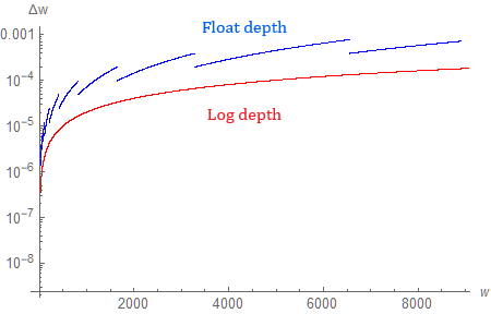
Zooming in, we can confirm that (in the limit of $f \to \infty$) a reversed floating-point Z-buffer is an approximation of a logarithmic depth buffer. It maintains the shape of the curve, but not its continuity. Nevertheless, it has a major performance advantage, since logarithmic depth cannot be linearly interpolated, which makes it less useful in practice.
Finally, what about the distance to the near plane? Does the old advice to place it as far as possible still hold true today? The answer is yes. In fact, for both floating-point and logarithmic depth buffers, precision scales linearly with the distance to the near plane. This implies that setting the near plane to 1/1000 instead of 1/10 reduces the effective resolution by a factor of 100 across the entire viewing range. Intuitively, the reason for this is because both Z-buffering techniques attempt to maintain (approximately) constant relative precision. Therefore, the smaller the distance, the higher the precision requirements, quickly consuming precious bits of storage. Floating-point number encoding (briefly explored at the beginning of this section) is another example of such behavior.
Conclusion
There are two ways to configure a reversed floating-point Z-buffer. Setting the far plane to a distance of 10000 meters results in a nearly constant (sub-millimeter if the near plane is 0.1 meters away) level of precision throughout the entire viewing range (except for the regions located next to the near and far planes, where the depth resolution rapidly increases). Pushing the far plane to infinity maintains (linear) precision in the near field (up to around 1000 meters for my setup), after which point it falls off linearly with distance. Infinite reversed floating-point Z-buffering can thus be seen as quasi-logarithmic. The distance to the near plane is still very important and should be set as high as possible.
A big caveat is that this article only considers Z-buffer precision. Everything has been calculated using infinite-precision arithmetic. There is no transformation pipeline, no rounding error, and no interpolation. These are the things that will likely cause more issues in practice.
Acknowledgments
I would like to thank Nathan Reed for reviewing this blog post and offering thoughtful comments.